Judge the differences among model file size, runtime memory, context length, and active parameters with real numbers.
Difficulty
Foundations
Structure
3 core units · 15 chapters
CORE UNIT 1 / 3
FP, quantization, and memory
Understand numerical representations and quantization errors, then budget actual memory for weights, cache, runtime and safety margin.
Difficulty
Beginner
Structure
Lessons 5 · Labs 2 · Assessment
Diagrams and tables: composed by the author using each lesson's official primary sources. Find the originals and review dates at the end of that lesson.
NEW HIRE ONBOARDING
Start in the order you would receive your first assignment
So that even a new hire with no prior IT background can follow along, we start with the situation, the task, the evidence, and when to report, before difficult definitions.
01
Read the situation in one sentence
If accumulated FP16 values become Inf or NaN during training, consider loss scaling or higher-precision accumulation; for inference, measure per-layer error and hardware kernel support.
02
Today's assignment
Understand numerical representations and quantization errors, then budget actual memory for weights, cache, runtime and safety margin.
03
Evidence that shows the work is complete
Do not target 100% VRAM use during normal operation. Measure peaks at the longest context and with concurrent requests.
04
When to stop and ask a senior colleague
BF16 retains the same 8-bit exponent range as FP32, but has fewer mantissa bits and thus lower precision.
Unpack unfamiliar terms first
FP16
A 16bit floating-point format with a 1bit sign, a 5bit exponent, and a 10bit mantissa
BF16
A 16-bit floating-point format that keeps the same 8-bit exponent range as FP32 and uses a 7-bit mantissa
Quantization
A technique that approximates high-precision values with limited codes and scales to reduce storage and computation costs
PREREQUISITE CHECK
Three things to check before reading
This is not a test of memorized answers. Think about each question first, then open the explanation to review the foundational concepts used in this course.
1How are bits and bytes related, and are GB and GiB the same unit?
1byte is 8 bits. GB usually means 1 billion bytes, while GiB means 1,073,741,824byte, so the same number of bytes is shown as different numbers. When comparing theoretical weight sizes with what a device reports, always state the unit.
2Does a file fitting on a storage device mean the same thing as it loading stably into memory at runtime?
They are not the same. Execution requires KV cache, runtime workspace, allocator reservations, and headroom for other processes in addition to model weights. Measure peaks at the longest context and target concurrency.
3What must be fixed to compare the quality of the two candidates fairly?
Pin model·tokenizer·chat template·runtime, prompt and sampling, input·output limits, evaluation data, and scoring criteria. Change only quantization to isolate the cause of differences.
TEXTBOOK GUIDE
Main text that covers each concept from its background to the criteria for judging it
We explain the material section by section so readers new to IT can connect causes and effects without memorizing terms.
CONCEPT FLOW
How the chapters connect
The chapters are not isolated short answers to memorize. Follow them from left to right to see how each chapter's concepts support the next decision.
1.Range and precision of FP32, FP16 and BF16→
2.Convert parameters × bits to bytes and GiB→
3.How quantization approximates values with scales and codes→
4.Read Q4_K_M and GGUF names conditionally→
5.Approve actual memory and quality together
FP, quantization, and memory: the overall map. If you lose track while reading the detailed explanations and chapters below, return to this sequence.
CONTROLLED EXPLANATION
Explore the order in which concepts build on each other
It does not start automatically. Play, or select the previous or next step, to see how the current concept connects to the next decision, step by step.
Current explanation · 1/5
Range and precision of FP32, FP16 and BF16
Both are 16bit, but FP16 and BF16 allocate bits differently between the exponent and mantissa, so their range and granularity differ.
FP16 uses less memory than FP32, but you must check for overflow of large values and rounding errors.
Up next: Convert parameters × bits to bytes and GiB, where this standard continues to apply.
See the full step description
1. Range and precision of FP32, FP16 and BF16
Both are 16bit, but FP16 and BF16 allocate bits differently between the exponent and mantissa, so their range and granularity differ. FP16 uses less memory than FP32, but you must check for overflow of large values and rounding errors.
2. Convert parameters × bits to bytes and GiB
Theoretical weight size is parameter count×average bits÷8; distinguish decimal GB, binary GiB, and the extra information in the actual file. A simple decimal calculation for 8B FP16 gives 16GB; expressed in binary units, the number is different.
3. How quantization approximates values with scales and codes
Quantization approximates continuous high-precision values using limited codes and scales, introducing rounding and clipping errors; range and block size affect results. Lower bit widths reduce storage and bandwidth but do not fully preserve the original values.
4. Read Q4_K_M and GGUF names conditionally
GGUF is a file format that holds metadata and tensors, and Q4_K_M is the name of a mixed quantization scheme in the llama.cpp ecosystem, so it cannot be reduced to a single 4-bit integer. Check format, quantization scheme and runtime support separately.
5. Approve actual memory and quality together
Add up the weight file, KV cache, runtime workspace, other processes, and safety headroom, and approve the candidate only when task regressions against a higher-precision baseline stay within the allowed range. Do not target 100% VRAM use during normal operation. Measure peaks at the longest context and with concurrent requests.
The text description below shows the same content without the animation. Your operating system's reduced-motion setting is also respected.Conceptual explanation 01
A numeric format is a contract that defines the range and spacing of values
Computers cannot store real numbers with infinite precision, so they divide a limited number of bits among the sign, the exponent that sets magnitude, and the significand or mantissa that sets significant digits. IEEE Floating Point 32 (FP32, 32-bit floating point) uses 1 sign bit, 8 exponent bits, and 23 mantissa bits. Floating Point 16 (FP16) uses 1, 5, and 10 bits, and Brain Floating Point 16 (BF16) uses 1, 8, and 7 bits. Although FP16 and BF16 are both 16-bit, they allocate different numbers of bits to the exponent and mantissa, so their range and spacing differ. Range and precision are not the same thing.
NVIDIA’s 2026 TensorRT accuracy documentation gives 65,504 as the largest finite FP16 value. Overflow beyond the representable range during computation can produce infinity (Inf), which may propagate to Not a Number (NaN) in subsequent operations. BF16’s 8-bit exponent supports a much wider range, but its 7 fraction bits can leave wider gaps between adjacent representable values than FP16 at the same magnitude. If training loss suddenly becomes NaN, locate the first overflow and check the accumulation type before focusing on the speed of 16-bit computation.
Being within the representable range does not guarantee adequate accuracy. A Unit in the Last Place (ULP) is the spacing between neighboring representable values at the current magnitude. Larger magnitudes can have wider spacing, rounding small differences away. Precision-sensitive operations include softmax, which amplifies small logit differences through exponentiation, reductions adding many values, and calculations around normalization. Test boundary inputs with large values, small differences and long accumulations instead of relying on one correct normal input.
Mixed precision does not assign one type to the entire model. Weight storage, activation, matrix-multiply inputs, accumulators, and outputs may use different types, with sensitive operations raised to FP32. Even for the same FP16 checkpoint, results and speed vary with which calculations the runtime and GPU kernels accumulate in wider formats. Do not infer all computation precision from the filename. Inspect the profiler, runtime precision report, and intermediate values from failing layers together.
Why does this happen?
The available bits are allocated between range and spacing, so equal storage size can still produce different overflow risks and rounding characteristics.
When is it a problem?
When training loss becomes Inf or NaN, or inference output repeats or collapses only on some large inputs, find the first abnormal operation under reduced precision.
Common beginner misconceptions
BF16 is not universally more accurate than FP16. It has a wider exponent range but lower mantissa precision.
How to verify it yourself
Run the same normal, large-value, and small-difference inputs with the FP32 baseline and the candidate precision, and record per-layer Inf·NaN, output differences, and kernel types.
Conceptual explanation 02
Connect parameter × bit calculations to bytes, GB, GiB, and actual files
The theoretical weight size is parameter count×bits per parameter÷8. If you simplify by assuming all 8 billion parameters are stored in 16bit, the result is 8,000,000,000×16÷8=16,000,000,000byte. At 4bit, it is 4,000,000,000byte. Multiplying parameters by bits gives the total number of bits, so divide by 8 to convert to bytes. The quick estimate “8B FP16 is about 16GB; 8B Q4 is about 4GB” is useful for screening candidates, but a theoretical value is not a guarantee for purchasing decisions.
Record units with numbers. Decimal gigabytes (GB, 1 billion bytes) and binary gibibytes (GiB, 2^30 bytes) differ. 16,000,000,000 bytes is 16GB but about 14.90GiB. Different units in file explorers, `ls`, and GPU tools can make one artifact appear to have different sizes. Record raw bytes and unit names together to avoid overestimating headroom by confusing 8GB of VRAM with a 7.45GiB display.
Actual quantized files store scales for each block or group and sometimes auxiliary values such as zero points or minima. Embeddings, output projections, normalization or quality-sensitive tensors may remain at higher precision; metadata, tensor-alignment padding and shard structure also occupy space. A Q4 label therefore need not mean exactly 4.000 average bits per weight. Inspect actual file bytes divided by parameter count and the tensor-type distribution to explain nominal bit width versus effective storage cost.
Consider a personal PC with a 4.8GiB 8B Q4 file and 6GiB VRAM. Do not stop at “1.2GiB remains.” GPU weights are accompanied by dequantization workspace, KV cache, graph and allocator reservations, and display VRAM. Short questions may run while an 8K context causes Out of Memory (OOM). Measure actual artifact bytes, memory immediately after startup, and peak memory for the longest input in sequence.
Why does this happen?
This is because the simple formula only calculates under the assumption that every parameter uses the same bit width, and does not include scale·mixed tensors·runtime state.
When is it a problem?
If a file saves but memory runs out during loading, or only short inputs pass and long contexts fail, the theoretical value was mistaken for the runtime requirement.
Common beginner misconceptions
A Q4 file does not necessarily mean exactly 4 bits per parameter, nor exactly 4GB for an 8B model.
How to verify it yourself
Record parameters·nominal bits·theoretical bytes·actual file bytes·average bits per weight·post-load memory and maximum-context peaks in the same table.
Conceptual explanation 03
How rounding and clipping errors arise between a scale and integer codes
In simplified symmetric uniform integer quantization, divide a real-valued weight by a scale, constrain it to the allowed integer range and round to the nearest code. Multiply the code by the scale to recover an approximation. With scale 0.1, 0.24 can be stored as code 2 and reconstructed as 0.2, while 0.26 can become code 3 and 0.3. Different original values can map to the same code, so quantization is not lossless compression.
Rounding error occurs when an original value between two representable values is moved to a nearby one. Clipping or clamping error occurs when a value outside the code range is cut to the maximum or minimum. NVIDIA TensorRT documentation explains the tradeoff: widening scale to reduce clipping may increase spacing and thus rounding error. A wider scale also has a cost.
Suppose a block contains mostly small values and one very large outlier. Widening the range to preserve the outlier can collapse several small values into the same code; narrowing it for small values clips the outlier. Effects differ by question and may appear first where small logit differences change choices: numerical-comparison boundaries, arithmetic, rare Korean proper nouns, code syntax and JSON closure.
Do not stop at one overall accuracy figure. Compare candidate tensors or logits against the FP16 baseline, and split task evaluation into normal, boundary and failure subsets. For example, an unchanged 95% average support-classification score does not justify production approval if errors double specifically at the refund refusal/approval boundary. Measure quantization error at both the numerical-loss and actual decision-loss levels.
Why does this happen?
Because the number of available codes is limited, several original values must map to the same approximation, or out-of-range values must be clipped to the boundary.
When is it a problem?
The average score can remain unchanged while wrong answers and format errors increase specifically for numbers, code, rare expressions and classification boundaries.
Common beginner misconceptions
It is wrong to think that dequantizing, like decompressing a file, can fully restore the original FP16 weights.
How to verify it yourself
Tabulate original values, scales, codes, reconstructed values, and errors for the same block, then add inputs with large errors to the task regression set.
Conceptual explanation 04
Where to place the scale: the whole tensor, each channel, or each group
Granularity describes how many values share one scale. Per-tensor uses one scale for the entire tensor, per-channel uses one per output channel, and per-group or per-block uses one for each fixed group of weights. A smaller sharing range can fit differing distributions and outliers better, but it increases the number of scales and the metadata, and weight packing and kernels must support that layout. Finer granularity is not always a free improvement.
Post-Training Quantization (PTQ) may use calibration samples or weight statistics to determine scales and protected components. The original GPTQ paper proposes one-shot weight quantization using approximate second-order information; AWQ uses activation distributions to identify important weight channels and protect them through scaling in a weight-only approach. Both may be labeled “4bit,” but their error-reduction criteria and required runtime kernels differ.
Calibration must represent the actual workload distribution but must not reuse the same data as the final evaluation set. For Korean customer inquiries, using only general English sentences to estimate importance may miss channels sensitive to Korean names or number formats. Conversely, including final test sentences in calibration can make evaluation-specific tuning look like generalization. Version calibration data containing normal, boundary, and failure cases separately from independent evaluation data.
Consider an incident in which, after a quantizer update, average perplexity improves but JSON keys in tool calls are often wrong. To recover, roll back to the previous artifact, then compare by changing only one of the quantizer revision, group size, calibration set, importance matrix, or runtime kernel. If only the name "the same Q4" is kept, the cause cannot be isolated. Store the quantization recipe itself as part of the model artifact.
Why does this happen?
Weight and activation distributions are uneven even within one tensor, so a single scale may not represent every region at the same quality.
When is it a problem?
If regressions appear only in specific languages, numbers, or JSON formats after applying a new group size or calibration data, check the recipe differences.
Common beginner misconceptions
A smaller group size does not guarantee better quality every time without file size or speed costs.
How to verify it yourself
Fix the quantizer revision, scheme, group size, calibration digest, importance matrix, average bits per weight, and downstream evaluation results for each candidate.
Conceptual explanation 05
Reading weight, activation, accumulator, and kernel support separately
Weight-only quantization mainly stores model weights in low bits and keeps activations in a wider type such as FP16 or BF16 during computation. Weight-and-activation quantization also reduces activations to types such as INT8 or FP8, which makes scale placement and calibration more important. An accumulator is an intermediate sum of multiple products, so it cannot be assumed to share the input type. The name “INT4 model” alone does not reveal which tensors and operations use which types.
Hugging Face's current bitsandbytes documentation illustrates this distinction. Linear8bitLt and Linear4bit replace ordinary linear layers with quantized alternatives, but other modules such as LayerNorm can use a separate dtype, and CPU-offloaded weights can remain FP32. Even when selecting NF4 storage, compute dtype can be configured separately. Record quantization configuration, device maps and per-module dtypes instead of relying only on the library name or load_in_4bit flag.
Speed is not determined by file size alone. If the GPU reads packed 4-bit weights and can efficiently dequantize and multiply them in a supported kernel, the memory-bandwidth burden drops and inference can become faster. Conversely, if the runtime does not support the architecture, group size, or tensor type, CPU fallback, conversion before execution, and kernel overhead at small batch sizes can make Q4 slower than Q8 or FP16. Lower-bit files are not always faster.
For example, a 7B Q4 model may fit in a laptop's integrated GPU memory, yet unsupported operators may move to the CPU, so the first token takes tens of seconds. On a desktop GPU, the same file may run quickly on dedicated kernels. The difference lies not in model intelligence but in hardware instructions, drivers, backend builds, and offload ratios. Instead of comparing only filenames and GPU product names, check the actual backend and layer placement in the runtime log.
A fair benchmark fixes model revision, prompt, context, output tokens, batch size, concurrency, sampling, and warm-up conditions. Record peak memory, Time to First Token (TTFT), prompt-processing tokens/s, generation tokens/s, power, and temperature separately. Do not equate one short generation or vendor peak TOPS with actual conversation speed. Compare performance and cost only among candidates that pass quality gates.
Why does this happen?
Computing with stored types requires unpacking, dequantization and accumulation, and device support for kernels that execute this path efficiently varies.
When is it a problem?
If a lower-bit candidate is actually slower, with CPU usage spiking and GPU usage low, check for fallback and the conversion path.
Common beginner misconceptions
Do not assume that using 4bit weights automatically makes activation·KV cache·accumulator 4bit as well.
How to verify it yourself
Record weight·activation·cache·accumulator types, offloaded layers, fallback operators, and actual token/s from runtime logs and profilers.
Conceptual explanation 06
Interpret GGUF and Q4_K_M names through metadata, tensor types, and tool versions
GGUF is a binary model format in the ggml ecosystem. The current official specification defines header magic and version, key-value metadata, each tensor's name, dimensions, type and offset, alignment padding and actual tensor data. It can contain metadata such as architecture, tokenizer, quantization version and license, but not every optional field is necessarily populated. A GGUF extension does not mean 4-bit quantization or a specific quality grade.
Q4_K_M is a llama.cpp name for a mixed configuration in the K-quant family. The official quantize tool offers `--pure` to disable mixing, as well as options to set separate quant types for output·token embeddings and specific tensors. A file with M in its name therefore does not mean every tensor uses the same 4-bit code. Only by checking the majority type label, such as `general.file_type`, and the actual type of each tensor can you explain “why a Q4 file is larger than expected.”
Record the original model ID, revision, and hash, converter and quantizer commits, input dtype, target quant type, group and importance-matrix settings, and output hash. Current llama.cpp documentation describes two steps: create a high-precision GGUF, then quantize. It states that `--allow-requantize`, which converts an already low-bit file again, can degrade quality far more than converting directly from 16-bit or 32-bit. Requantization is not the same as converting directly from the original.
If a runtime does not recognize a new architecture or tensor type, the problem may surface immediately as an unknown architecture, unsupported type, or load failure. A more dangerous case is when the file opens but the chat template or tokenizer metadata does not match, so answers repeat and the end token does not work. When recovering, return to the verified runtime build and original artifact bundle before papering over the problem with an arbitrary metadata override. Compare loader logs, GGUF metadata dumps, and the same regression prompts together.
Why does this happen?
A format is a container that holds various architectures, metadata, and tensor types, while quantization is the numeric representation recipe inside it, so they are different layers.
When is it a problem?
If unsupported tensor errors, CPU fallback, repeated output, or unexpected file sizes appear, cross-check the runtime, metadata, and tensor types against the conversion records.
Common beginner misconceptions
A `.gguf` extension or Q4_K_M in the name does not mean provenance, compatibility, and quality have been automatically verified.
How to verify it yourself
Store the original revision, converter/quantizer commit, command, metadata dump, tensor type distribution, hash, and runtime build in one manifest.
Conceptual explanation 07
Building a memory budget from weights to KV cache·workspace·safety headroom
Running a model requires more than the weights offloaded to the GPU: the KV cache that stores the Keys and Values of tokens already read, workspace for attention and matrix kernels, regions reserved by the graph and allocator, and memory used by the multimodal projector and other processes. With CPU offload, consider both budgets, system RAM and GPU VRAM, together with transfer latency between the two devices. Do not treat disk file size and runtime peak as the same value.
Longer Context and more concurrent sequences increase KV cache. Even with the same model and weight quantization, one 2K question and two concurrent 32K documents have very different requirements. Cache dtype may be independent of weight dtype: Q4 weights do not automatically make KV cache 4bit. Validate a product's maximum-context figure by measuring required cache and prompt-processing time on actual equipment at that context.
When Out of Memory occurs, first save model·quant·runtime·driver, context·maximum output·concurrent requests, GPU allocated·reserved memory, and system RAM from immediately before the error. Establish a small baseline with 1 concurrent request and shorter context·output reservation, then change one variable at a time. If it still fails, consider offload, a smaller model, or lower bit width. Do not immediately restore the original load merely because execution succeeds; compare peaks and latency.
If an 8B Q5 on a 12GB GPU starts hitting OOM after a runtime update, do not immediately switch to Q3. Rerun the same inputs on the previous runtime and inspect allocator/workspace changes. Recover with reduced context, then change only the update or quantization to isolate causes. VRAM at 100% is not a stable operational target; leave room for input variation and monitoring tools.
Why does this happen?
Besides reading weights, generation stores past token state and intermediate values, so memory varies with input length and concurrency.
When is it a problem?
If short questions work but long documents, concurrent requests or runtime updates cause OOM, measure the memory budget beyond weights.
Common beginner misconceptions
A file smaller than VRAM does not mean it runs stably at every context length and under concurrent requests.
How to verify it yourself
Repeatedly measure usage immediately after loading, prefill peaks, generation peaks and system RAM across minimum, representative and longest inputs at concurrency 1 and the target value.
Conceptual explanation 08
Approve candidates using a high-precision baseline and task-regression gates
First, pin the high-precision baseline's exact model revision, tokenizer, chat template, runtime, and prompt. In the candidate, change only quantization and use identical normal, boundary, and failure inputs, sampling seeds, and output limits. If a task has no single correct answer, have at least two people review blindly against a rubric with model names hidden. Score evidence, omissions, format, and safety separately so shorter quantized-model answers do not score higher by accident.
Set approval criteria before seeing results: for example accuracy loss at most 1 percentage point, JSON compliance at least 99.5%, zero additional dangerous answers, peak-memory reduction at least 25%, and p95 first-token latency at most 2 seconds. Hold a candidate that passes memory requirements but fails format compliance. Lowering thresholds after results turns numbers into decoration for a chosen conclusion rather than a gate.
Do not let one average hide subset failures. Overall accuracy across 500 cases can remain unchanged while errors rise sharply in 50 cases involving long numbers, code, rare Korean names, long context and tool schemas. Set minimum passing thresholds for each subset and add failing sentences to a regression corpus. Review wrong answers and duplicates in the evaluation data itself to avoid confusing quantization loss with an incorrect answer key.
Finally, test the rollback for real. Stop the candidate artifact, redeploy the previous hash, runtime, and template bundle, and confirm that the same failing inputs recover. The approval record keeps the source revision, quant recipe, file hash, evaluation results, peak memory, measurement hardware, known limitations, and owner. The lab enters baseline and candidate figures to perform a failure→criteria-met recovery, but those browser results do not replace evidence from actual model tests.
Why does this happen?
Quantization benefits and losses vary by model, task and runtime, so file sizes or public averages alone cannot predict your deployment results.
When is it a problem?
Promotion is not allowed if important boundary inputs or JSON formats regress, or rollback artifacts cannot be reproduced, even when the average is unchanged.
Common beginner misconceptions
A small perplexity change or a model that loads normally does not automatically mean that real task quality is unchanged.
How to verify it yourself
Run the pre-agreed per-subset quality, format, safety, memory, and latency gates on the same evaluation set, and record recovery to the previous artifact as well.
Conceptual explanation 09
Manage personal equipment selection and operational changes under one quantization contract
When choosing a personal PC, first write down the work you will actually do rather than asking “how many B can it run?” Distinguish whether you ask a few short questions a day, want it to read a 50-page document at once, need low latency as in code completion, or need speech and images. Then calculate the memory required for the model revision and quant candidate, the context, and 1 concurrent sequence. Being able to run is different from being usable every day. If fan noise, power, heat, and first-token latency exceed what your daily environment can tolerate, the configuration is not suitable even if it fits in memory.
When comparing 7B Q4 and Q5 on an 8GB-VRAM laptop, do not choose solely because public averages show slightly better Q5 quality. Repeatedly measure peaks, first-token latency, sustained generation speed and temperature with the same Korean documents and output lengths. Q4 may be more stable if Q5 throttles after a few minutes or lacks headroom at target context. Conversely, if Q4 product-code and number errors exceed limits, compare a smaller model at higher precision too.
For a small team's API, inspect simultaneous requests and longest inputs rather than one average request. Even with 20% headroom in a single-user test, overlapping KV caches and scheduler workspaces from four requests can cause OOM. Send only some traffic to new quantized candidates and monitor errors, queues, p95, peak memory and subset quality. If failures increase, roll back to the previously verified artifact and isolate load and quality causes instead of automatically lowering bit width.
Purchase and deployment records can share one table. Record required tasks and failure costs, model, tokenizer, and template revisions, quantization schemes and groups, actual file bytes, runtime, drivers, hardware, context, concurrency, quality and format gates, peaks, latency, power, temperature, licenses, and rollback locations. If many fields are blank, it is too early to decide on a bigger GPU or smaller file. Combine equipment-price comparisons with model benchmarks to see total cost and risk.
Quantization changes are also production deployment changes. New converter versions or changes to calibration data, importance matrices, group sizes, cache dtypes, or kernels make a new candidate even with the same Q4 label. Re-run the same evaluations and load tests and update known limitations. This avoids both “smaller is better” and “higher precision is safe,” helping select the simplest recoverable combination that meets quality criteria.
Operational reports preserve more than successful numbers: record failing inputs, quality costs of memory savings, held candidates and rollback reasons. These records help decide whether to retry lower precision, add hardware to retain higher precision, or change context/concurrency requirements. Deleting failures repeats tests of the same quantization under different names and rediscovers errors through users. Retain reproducibility conditions and retirement reasons even for unapproved candidates, plus retest dates and additional evidence needed.
Why does this happen?
Practical results depend jointly on model weights, context, concurrency, sustained runtime/device performance and acceptable task error.
When is it a problem?
It may run once, yet slow down over extended use, hit OOM with multiple users, or show different quality with the same Q4 after a tool update.
Common beginner misconceptions
There is no single ranking in which the lowest bit width is always efficient or the highest precision is always best.
How to verify it yourself
Repeatedly measure sustained load·noise·temperature for personal equipment, and target concurrency·queue·p95·rollback for team servers, alongside the same quality evaluation.
CONCRETE CASES
Check concepts in different situations
Before memorizing definitions, compare how these concepts appear on a personal PC and in real work.
Case 1 · Range and precision of FP32, FP16 and BF16
If accumulated FP16 values become Inf or NaN during training, consider loss scaling or higher-precision accumulation; for inference, measure per-layer error and hardware kernel support.
Key points to check here: FP16 uses less memory than FP32, but you must check for overflow of large values and rounding errors.
Case 2 · Convert parameters × bits to bytes and GiB
8,000,000,000×4÷8 is 4,000,000,000byte, which a file system shows as about 3.73GiB, and actual Q4 files differ because of scale·metadata.
Key points to check here: A simple decimal calculation for 8B FP16 gives 16GB; expressed in binary units, the number is different.
Case 3 · How quantization approximates values with scales and codes
Widening the scale to fit one large outlier in a block can collapse small values into the same code, which makes per-channel or per-group scaling and the calibration method important.
Key points to check here: Lower bit widths reduce storage and bandwidth but do not fully preserve the original values.
Case 4 · Read Q4_K_M and GGUF names conditionally
When choosing a Q4_K_M file, record base model·revision·converter commit·quant method·imatrix·tensor mixture·hash and your runtime’s support together.
Key points to check here: Check format, quantization scheme and runtime support separately.
Case 5 · Approve actual memory and quality together
If 8B Q4 runs for short questions on an 8GB GPU but hits OOM with a 32K context and two concurrent requests, lower the context·concurrency·cache type to establish a baseline, then raise one item at a time.
Key points to check here: Do not target 100% VRAM use during normal operation. Measure peaks at the longest context and with concurrent requests.
CHAPTER 1 / 5
Range and precision of FP32, FP16 and BF16
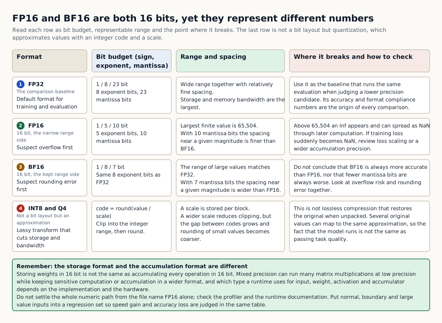
Floating point (FP) represents very large and very small numbers using a sign, an exponent, and a significand, also called a mantissa. FP32 uses 1 sign bit, 8 exponent bits, and 23 fraction bits, providing a wide range and relatively fine spacing. FP16 uses 1, 5, and 10 bits, respectively, for 16 bits in total, reducing storage and memory bandwidth but narrowing the exponent range. NVIDIA’s TensorRT accuracy documentation identifies 65,504 as the largest finite FP16 value and warns that overflow in operations exceeding the representable range can produce Inf, which may propagate to NaN in subsequent calculations.
Brain Floating Point 16 (BF16) uses 1 sign bit, 8 exponent bits, and 7 mantissa bits. It has the same exponent-bit count as FP32 and a broad range, but fewer mantissa bits than FP16 and wider spacing near values of the same magnitude. Do not conclude that BF16 is always more accurate than FP16 or always worse because it has fewer mantissa bits. Consider overflow risk, rounding errors, per-operation accumulation, and hardware support together.
Storing weights in 16bit is also different from accumulating every operation in 16bit. Mixed precision can run many matrix multiplications at lower precision while keeping sensitive calculations or accumulations in a wider format. Which types a runtime uses for inputs·weights·activations·accumulators depends on the implementation and hardware. Do not assume the entire numeric path from “FP16” in a filename alone; check the profiler and the runtime documentation.
Real symptoms range from subtle quality loss to obvious errors. Logits may change sharply or outputs may repeat on only some inputs, and during training the loss may suddenly become NaN. When recovering, before switching every layer to FP32, find the failing input and the first abnormal layer, and compare against a candidate that keeps only sensitive computations at higher precision. Add normal, edge-case, and large-value inputs to the regression set and weigh speed gains against accuracy loss in the same table.
How to read the figure The total bit count does not determine the format. FP16’s largest finite value is 65,504, and arithmetic overflow can produce Inf. BF16 preserves a wide exponent range at the cost of wider spacing between significand values. INT8 and Q4 use lossy approximations based on a scale and integer codes.
To recap the key points
FP16 uses less memory than FP32, but you must check for overflow of large values and rounding errors.
BF16 retains the same 8-bit exponent range as FP32, but has fewer mantissa bits and thus lower precision.
How this connects in practice
If accumulated FP16 values become Inf or NaN during training, consider loss scaling or higher-precision accumulation; for inference, measure per-layer error and hardware kernel support.
CHAPTER 2 / 5
Convert parameters × bits to bytes and GiB
The first calculation, covering weights only, is parameter count×bits per parameter÷8. Simplifying an 8B model to FP16 gives 8 billion×16bit÷8=16 billion bytes, or 16GB in decimal notation. For 70B, the same method gives 140GB. This is a theoretical value that assumes every uncompressed parameter uses exactly 16bit, and it does not include checkpoint shard metadata, alignment, duplicate storage, or adapters·projectors.
Distinguish GB from GiB. Storage manufacturers and many model descriptions use 1GB = 1 billion bytes, while operating systems and tools may use 1GiB = 1,073,741,824 bytes. That is why the same 16,000,000,000 bytes can appear as 16GB or about 14.90GiB. Writing just "16 gigs" without a unit introduces an error of several percent when comparing file size with VRAM, and with little headroom that can change the decision.
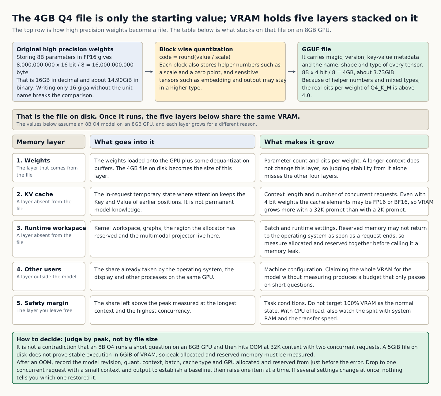
The 4bit theoretical value is likewise 8B×4÷8=4GB, but the actual quantized file does not have to be exactly 4GB. Each block stores auxiliary numbers such as a scale and a zero point or minimum value, and embedding·output·some sensitive tensors may be kept in a higher-precision type. The table in the llama.cpp quantize documentation also reports Q4_K_M not as a plain 4.0 but as a specific bits per weight and file size. Those values are examples for a particular model·commit·test setup and should not be copied as-is to other architectures.
The first lab calculates a starting value for weights from parameters and nominal bits, then adds the KV cache, runtime buffers, and a safety margin. A result below VRAM is not an immediate success; measure the actual artifact's bytes and peak allocated and reserved memory. Record step by step whether the file fits on disk, whether it can be read into system RAM, how much is offloaded to the GPU, and what the peak is at the longest context with concurrent requests.
To recap the key points
A simple decimal calculation for 8B FP16 gives 16GB; expressed in binary units, the number is different.
Average bits per weight includes block scales and some high-precision tensors, so it may exceed the nominal 4 bits.
How this connects in practice
8,000,000,000×4÷8 is 4,000,000,000byte, which a file system shows as about 3.73GiB, and actual Q4 files differ because of scale·metadata.
CHAPTER 3 / 5
How quantization approximates values with scales and codes
In a simplified integer-quantization process, divide the original floating-point value by a scale, clip it to the allowed integer range, then round to obtain a code. Dequantization multiplies the code by the scale to recover an approximation. Values between codes incur rounding error; values outside the allowed range incur clipping error at the boundary. Increasing the scale reduces clipping but widens code spacing, making rounding of small values coarser.
Per-tensor quantization uses one scale for an entire tensor, per-channel uses one for each output channel, and per-group or per-block uses one for each fixed group of weights. These methods differ in metadata overhead and error characteristics. Large outliers in the weight distribution can pull the entire range toward their values. GPTQ proposed one-shot weight quantization without retraining from scratch, while AWQ proposed identifying and protecting important weight channels using activation statistics. Read reported paper results in the context of the specific model, hardware, and kernel conditions.
Weight-only quantization stores model weights at lower bit widths while activations may use higher-precision computation. Quantizing both weights and activations makes calibration data and Q/DQ placement more important. Static quantization uses predefined scales; dynamic quantization may determine some scales from runtime inputs. The label “INT4 model” alone does not identify which tensors and activations use which granularity.
Quantization differs from lossless compression that recovers the original exactly. Multiple original values may map to the same low-bit approximation, losing information. A valid file hash and a running model therefore do not establish task-quality approval. Compare the high-precision baseline and candidate on fixed sensitive cases such as classification boundaries, long numbers, code, rare Korean proper names, and JSON formats.
To recap the key points
Lower bit widths reduce storage and bandwidth but do not fully preserve the original values.
Weight-only, weight-plus-activation, static, and dynamic quantization are different paths.
How this connects in practice
Widening the scale to fit one large outlier in a block can collapse small values into the same code, which makes per-channel or per-group scaling and the calibration method important.
CHAPTER 4 / 5
Read Q4_K_M and GGUF names conditionally
GGUF is a format containing metadata, tensor names, shapes and types, and binary data so GGML-based runtimes can read a model. The official specification defines magic, version, key-value metadata, tensor information and data sections. The GGUF extension does not mean a quality grade or 4-bit quantization. The same format can contain F32, F16, BF16, Q4_K and other types, as well as tokenizer and architecture metadata.
Read Q4 in Q4_K_M as roughly 4bit K-quant and M as a mixed configuration in the llama.cpp ecosystem. It does not mean every tensor is stored as pure 4bit codes. llama.cpp’s quantize tool provides options for separate output or embedding types and per-tensor types. Check GGUF metadata, tensor-type distributions, and converter·quantizer versions, not just the filename.
Requantization is the process of converting an already approximated low-bit file into another low-bit format. Information lost in the first quantization cannot be restored, so additional rounding and clipping errors can accumulate. The official llama.cpp quantize documentation also warns that `--allow-requantize` can degrade quality far more than converting directly from a 16bit·32bit original. Whenever possible, convert directly to the target format from a verified high-precision original at the exact revision.
Runtime compatibility is a separate gate. Even with the same Q4_K_M label, an older runtime may not recognize a new architecture, GGUF metadata version, or tensor type. Symptoms include unknown architecture·unsupported tensor type·incorrect tokens or CPU fallback. Before blaming files, record runtime commits and build backends, model metadata, and converter logs together; return to an officially supported combination for a baseline.
How to read the figure The size of a Q4 file is only the first layer of run time memory. A short question may pass on an 8GB GPU while 32K context with two concurrent requests changes the peak, so judge by the peak allocated value rather than by file size.
To recap the key points
Check format, quantization scheme and runtime support separately.
Requantizing an already quantized file can damage quality more than direct conversion from original high-precision weights.
How this connects in practice
When choosing a Q4_K_M file, record base model·revision·converter commit·quant method·imatrix·tensor mixture·hash and your runtime’s support together.
CHAPTER 5 / 5
Approve actual memory and quality together
Runtime memory includes more than weights. Add GPU-resident weights and dequantization buffers, attention KV cache, kernel workspace, graph·allocator reservations, multimodal projectors, OS·display, and other processes. With CPU offload, inspect system-RAM/GPU-VRAM distribution, transfer speed, and page faults. A 5GiB disk file alone does not establish stable execution in 6GiB VRAM.
When Out of Memory (OOM) occurs, record the model revision, quant, context, batch·concurrent sequences, cache type, GPU allocated·reserved memory, and system RAM from immediately before the error. Confirm a baseline with a single concurrent request and a smaller context and maximum output; if it still fails, consider a smaller model or lower weight bits. Once it runs, increase context, output, and concurrency one at a time to set the safety margin. If you change several settings at once, you cannot tell which change produced the recovery.
After reducing memory, run the same evaluation as the high-precision baseline. Use accuracy, evidence faithfulness, format compliance, hallucination and safe refusal as quality metrics, and peak memory, first-token latency and generation speed as performance metrics. Inspect code, math, numbers, rare languages, long contexts and tool schemas as subsets instead of relying on one average. A candidate with the same average but more JSON-closure failures may be unsuitable for automation.
The second lab uses measured baseline and quantized-candidate results to judge allowable accuracy loss, minimum format compliance, and memory reduction together. Lowering criteria after the fact to make the numbers pass turns evaluation into decoration rather than a gate. Set criteria before deployment, preserve failed candidates and results, and test a rollback path for returning immediately to the previous artifact.
To recap the key points
Do not target 100% VRAM use during normal operation. Measure peaks at the longest context and with concurrent requests.
Smaller files and faster token generation do not automatically justify losses in accuracy, supporting evidence or format compliance.
How this connects in practice
If 8B Q4 runs for short questions on an 8GB GPU but hits OOM with a 32K context and two concurrent requests, lower the context·concurrency·cache type to establish a baseline, then raise one item at a time.
INTERACTIVE LAB 1 / 2
Lab 1 · Weight memory calculator
Enter values in the browser and check the execution results and the failure and recovery paths. No commands are ever sent to real equipment or the NAS.
Calculating from theoretical weight size to a runtime memory safety line
Before seeing results, enter the model, precision, KV cache, and available memory. If the configuration fails, change one condition at a time to find a runnable baseline.
Situation
The longest context was assumed to run merely because the Q4 file was smaller than GPU memory.
Goal
Distinguish the theoretical weight size from the execution budget, which includes runtime·cache·headroom.
Prerequisites
Prepare the model parameters, candidate quant, usable memory on the actual hardware, and a cache estimate for the target context.
Success criteria
Explain that the estimated execution budget is at most 90% of available memory and that actual peaks must be remeasured.
Enter parameter count, weight bit width, and expected KV cache.
Enter the memory actually available, excluding other processes.
Memory budget calculation: run it, and if it fails, change only one of context, model, or bit width and run it again.
Limitations and recovery: This educational approximation adds a 15% weight allowance, 1.25GB for runtime and the user-entered cache. High-precision tensors, backend workspace and OS usage vary, so measure actual loading, prefill and generation peaks and return to previous settings on failure.
INTERACTIVE LAB 2 / 2
Lab 2 · Quantization regression approval lab
Enter values in the browser and check the execution results and the failure and recovery paths. No commands are ever sent to real equipment or the NAS.
Approve quantized candidates through quality, format, memory and rollback checks together
Enter actual measurements for the high-precision baseline and candidate. A candidate qualifies for deployment only after passing every gate defined before results were seen.
Situation
The Q4 candidate reduced memory, but regressions in Korean classification and JSON format have not been checked.
Goal
Evaluate accuracy, format compliance, peak memory, and artifact provenance and rollback as a single approval condition.
Prerequisites
Prepare baseline and candidate results measured using the same model, prompt, and evaluation set, the conversion manifest, and the previous artifact.
Success criteria
Pass every numerical gate and verify direct conversion from the high-precision source and a rollback retest.
Before viewing candidate results, enter the allowed accuracy drop, minimum format compliance, and memory reduction criteria.
Enter baseline·candidate measurements under the same evaluation conditions and two change-management items.
Run the approval gate Then read the hold reasons, strengthen the candidate or evidence, and rerun.
Evidence limits: Entered numbers stay in the browser and do not run an actual model. A passing screen in this lab cannot replace model hashes, original evaluation data, runtime logs, or actual rollback records.
KEY TERMS
Key terms in this unit
FP16
A 16bit floating-point format with a 1bit sign, a 5bit exponent, and a 10bit mantissa
BF16
A 16-bit floating-point format that keeps the same 8-bit exponent range as FP32 and uses a 7-bit mantissa
Quantization
A technique that approximates high-precision values with limited codes and scales to reduce storage and computation costs
GGUF
A binary file format defined by the ggml ecosystem to hold metadata and model tensors of multiple types
UNIT WORKBOOK
Exercises and worksheets for applying concepts to new situations
Start by checking basic principles, then expand to practical workplace decisions. After submitting an answer, you can see why every option is correct or incorrect, not just the correct answer.
Basic Question 1
What is the most accurate explanation of the difference between FP16 and BF16?
Basic Question 2
Assuming for simplicity that all weights of an 8B model are stored in 4 bits, what best describes the relationship between that theoretical value and the actual file?
Apply Question 3
On a device with 6GiB VRAM, a 4.8GiB Q4 file runs for short questions but hits OOM on a 16K document. What is the safest diagnosis and recovery?
Other programs' usage and the number of concurrent requests on the same machine have not been recorded yet; the only known fact is that weight quantization is Q4.
Apply Question 4
With only a Q5 file on hand and a need to produce Q4_K_M quickly, what is the most reasonable decision?
The original BF16 revision can be obtained again, but there is no quantizer version or calibration record for the current Q5 file.
Capstone Question 5
What is the most complete plan for promoting a Q4 candidate to production from an FP16 baseline?
It is used for Korean support classification and JSON tool calls; memory reduction, p95 latency and format compliance all matter.
PERSONAL WORKSHEET
A learning worksheet you adapt to your own environment
Your input remains only on the current browser screen and is not stored or transmitted externally. Use categories and pseudonyms instead of actual sensitive information.
OFFICIAL SOURCES
Verify against official sources
Technical, compatibility, and model information reviewed: August 2026
Calculate one request’s token budget and KV cache growth from the actual config, and recover from memory shortages under long contexts and concurrent requests, starting from a small baseline.
Difficulty
Foundations
Structure
Lessons 5 · Labs 2 · Assessment
Diagrams and tables: composed by the author using each lesson's official primary sources. Find the originals and review dates at the end of that lesson.
NEW HIRE ONBOARDING
Start in the order you would receive your first assignment
So that even a new hire with no prior IT background can follow along, we start with the situation, the task, the evidence, and when to report, before difficult definitions.
01
Read the situation in one sentence
With an 8,192-token limit, a request exceeds the limit if hidden input and reserved output bring the total to 8,800 tokens, even when the visible question is only 400 tokens.
02
Today's assignment
Calculate one request’s token budget and KV cache growth from the actual config, and recover from memory shortages under long contexts and concurrent requests, starting from a small baseline.
03
Evidence that shows the work is complete
Measure weights, cache, workspace, allocator, and other processes as a single total.
04
When to stop and ask a senior colleague
Distinguish official maximums from the practical limits of your runtime, hardware, and tasks.
Unpack unfamiliar terms first
Context window
Range of tokens that can be processed in one request
Key-Value cache(KV cache)
Memory storing intermediate attention results for previous tokens and reusing them when generating the next token
Out of Memory(OOM)
Execution halted because the required data cannot fit in available GPU or system memory
PREREQUISITE CHECK
Three things to check before reading
This is not a test of memorized answers. Think about each question first, then open the explanation to review the foundational concepts used in this course.
1Is the question visible in the input box the only thing that uses context?
No. System instructions, role tokens, conversation history, retrieved documents, tool schemas, the question, and newly generated output all share the same context budget. Measure the completed prompt with the tokenizer immediately before the model call.
2Is the model file size the same as the GPU memory required at runtime?
They are not the same. Execution requires space for KV cache, kernel workspace, graph and allocator reservations, and other processes in addition to weights. More context and concurrent sequences increase cache size even when the file remains unchanged.
3Is the number of query heads in attention always equal to the number of KV heads?
The counts can be equal in MHA, but in GQA and MQA multiple Query heads share fewer Key·Value heads. Use num_key_value_heads from the exact config for cache calculations.
TEXTBOOK GUIDE
Main text that covers each concept from its background to the criteria for judging it
We explain the material section by section so readers new to IT can connect causes and effects without memorizing terms.
CONCEPT FLOW
How the chapters connect
The chapters are not isolated short answers to memorize. Follow them from left to right to see how each chapter's concepts support the next decision.
1.Read the context window as a budget that includes input you cannot see on screen→
2.Prefill·decode and the KV cache lifecycle→
3.Calculate KV cache bytes from the config→
4.Convert cache strategy and concurrent requests into an operating budget→
5.Recover from Out of Memory at a small baseline and lock it in as the operating limit
Context and KV cache: the overall map. If you lose track while reading the detailed explanations and chapters below, return to this sequence.
CONTROLLED EXPLANATION
Explore the order in which concepts build on each other
It does not start automatically. Play, or select the previous or next step, to see how the current concept connects to the next decision, step by step.
Current explanation · 1/5
Read the context window as a budget that includes input you cannot see on screen
The total token budget a model can use in one request; hidden inputs and new output consume it along with the user's question.
Sum system text, template, history, retrieved documents, tools, question, and reserved output using one consistent unit.
Up next: Prefill·decode and the KV cache lifecycle, where this standard continues to apply.
See the full step description
1. Read the context window as a budget that includes input you cannot see on screen
The total token budget a model can use in one request; hidden inputs and new output consume it along with the user's question. Sum system text, template, history, retrieved documents, tools, question, and reserved output using one consistent unit.
2. Prefill·decode and the KV cache lifecycle
Reuse already computed Keys·Values during prefill, which reads the whole prompt at once, and decode, which generates the next token one at a time. The cache is not permanent model knowledge; it is intermediate attention state kept for the duration of a request.
3. Calculate KV cache bytes from the config
A first approximation of a standard decoder cache is 2×layer×KV head×head dimension×token×byte×sequence; record the source and exceptions for each value. Check `num_key_value_heads` and the actual cache dtype, rather than Query head count.
4. Convert cache strategy and concurrent requests into an operating budget
Dynamic, static, sliding, offloaded, and quantized caches each make different trade-offs among memory, compilation, transfer, conversion, and latency. Do not look only at average length; measure with the actual distribution, which mixes short conversations and the longest documents.
5. Recover from Out of Memory at a small baseline and lock it in as the operating limit
Recover from OOM by preserving error conditions, establishing concurrency 1·short-context baselines, increasing one variable at a time, retesting the same failing input, and rolling back. Measure weights, cache, workspace, allocator, and other processes as a single total.
The text description below shows the same content without the animation. Your operating system's reduced-motion setting is also respected.Conceptual explanation 01
A context window is a per-request token budget, not a count of characters on screen
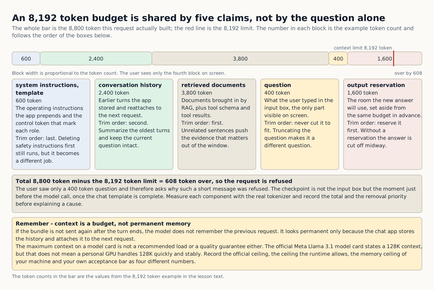
A context window is the maximum range of tokens a model can consult together in a single request. It does not count only the question the user types into the input box. System instructions that the application prepends, control tokens that mark roles, previous conversation, documents fetched by Retrieval-Augmented Generation (RAG), tool schemas and results, the current question, and the newly generated answer all draw on the same budget. If this bundle is not sent again, the model does not automatically remember an earlier request. It only looks like permanent memory because the chat app saves the history and attaches it to the next request.
With an 8,192-token limit, allocating 600 to system/template, 2,400 to history, 3,800 to retrieved documents, 400 to the question, and 1,600 to output totals 8,800, already 608 tokens over budget. The user sees only a 400-token question and may wonder why it was rejected. The checkpoint is not the input box but the completed chat-template prompt immediately before the model call. Count each component with the actual tokenizer and reserve output space first to prevent truncated answers.
The maximum context number on a model card does not guarantee recommended usage or quality for your task. Meta’s official Llama 3.1 model card specifies 128K context, but that number does not mean a personal GPU processes 128K quickly and reliably or that important conditions are never missed in long Korean texts. Longer inputs increase prefill computation time and KV cache, and irrelevant sentences can crowd out important evidence. Record the official limit, the runtime limit, your hardware’s memory limit, and the task pass line as separate values.
For personal document summarization, rather than always inserting an entire file, preserve the titles and section structure to find the parts you need; in a small team's support app, summarize older conversation turns while preserving the current question and safety instructions. If you handle overflow by deleting system rules first or arbitrarily truncating the question, the request may run, but it becomes a different task. Only by deciding the trimming priority in advance and rechecking quality against the same questions·reference answers can you keep context savings from turning into simple information loss.
How to read the figure The 400 token question in the input box is only one share of the whole budget. Set the output reservation aside first, then trim the unrelated retrieved documents and the oldest conversation history.
Why does this happen?
This is because the application merges off-screen inputs and generated output extends the same sequence, so the character count the user sees differs from the token count the model processes.
When is it a problem?
Check final prompt composition and reserved output space when short questions exceed context limits, answers are truncated, or requests suddenly get rejected as conversations grow longer.
Common beginner misconceptions
A longer Context does not mean the model is smarter or permanently remembers previous conversations.
How to verify it yourself
Measure system text, template, history, retrieved documents, tools, question, and reserved output separately using the actual tokenizer. Record the total and removal priorities.
Conceptual explanation 02
How KV cache reduces repeated computation in prefill and decode
Autoregressive generation builds answers one token at a time. Prefill processes the full prompt, computing Queries, Keys, Values, and attention from hidden states at each position. During decode, each new position’s Query attends to previous positions’ Keys and Values. Recomputing those previous values repeats matrix operations and wastes more work as answers grow. The Key-Value cache stores these attention intermediate values for reuse.
As an analogy, instead of re-summarizing every attendee's remarks from the start each time a new sentence is written in long meeting minutes, you keep stacking an index table for each remark alongside. When a new sentence appears, you add only that sentence's table and refer to the earlier ones. This reduces computation, but the index tables themselves take up space. Just as the tables grow when a conversation is long or several users' minutes are kept at once, cache memory grows as the number of tokens and sequences increases.
KV cache has a different lifecycle from model weights. Even with the same Q4 weight file, the cache can grow when the prompt increases from 2K to 32K, and 4-bit weights do not automatically make the cache 4-bit. Depending on the runtime and settings, the cache dtype may be FP16, BF16, or a quantized type. That is why the downloaded file size and the GPU memory growth during a long conversation show different numbers. An unchanged disk file is evidence neither that there is no memory leak nor that the cache is small.
Disabling the cache may reduce memory use, but recomputing past Keys and Values at every decode step can greatly reduce speed. Hugging Face's official documentation describes caching as a way to reduce repeated computation and improve generation response. Disabling it unconditionally may help a small reproduction test, but is not the default remedy for normal operations. Measure actual latency together with cache release behavior and whether the memory allocator retains reusable space after a request ends.
Why does this happen?
The next token refers to the attention state of all preceding tokens, so storing past Keys and Values avoids repeating the same projection calculations.
When is it a problem?
If memory keeps growing during long generation or token generation slows sharply after disabling the cache, you are observing the tradeoff between storage and repeated computation.
Common beginner misconceptions
KV cache is neither a model's permanent knowledge nor a conversation database; it is runtime memory that temporarily holds a request's attention state.
How to verify it yourself
With the same prompt and output length, record peak memory, prefill time, decode token/s, and the memory change after requests end, with and without the cache.
Conceptual explanation 03
Calculate the cache from layers, KV heads, head dimension, tokens, bytes, and sequences
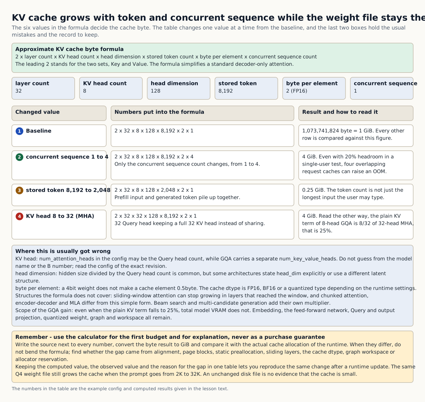
A simplified KV cache byte formula for standard decoder-only attention is `2 × number of layers × number of KV heads × head dimension × number of stored tokens × bytes per element × number of concurrent sequences`. The leading 2 represents the two sets, Key and Value. Plugging in 32 layers, 8 KV heads, head dimension 128, 8,192 tokens, 2 bytes per element for FP16, and 1 sequence gives 2×32×8×128×8,192×2=1,073,741,824 bytes, or 1GiB. Keeping 4 sequences at once under the same conditions makes the simple cache term 4GiB.
KV-head count is the most frequently mistaken value. `num_attention_heads` may count Query heads; Grouped-Query Attention (GQA) has a separate `num_key_value_heads`. Hidden size divided by Query-head count is a common head dimension, but some architectures explicitly define `head_dim` or use latent structures. Check the exact revision's configuration and implementation instead of guessing from names or B counts.
Token count is not just the maximum length entered by a user. Prefill inputs and generated tokens accumulate together in the cache, and sequences within a batch may be managed with padding or separate pages. Beam search or multiple candidates may multiply cache requirements differently from a single sequence. Sliding-window attention may stop cache growth in layers that reach the window size. Chunked attention, encoder-decoder architectures, and Multi-head Latent Attention (MLA, which represents Keys and Values in a smaller latent space) differ from the simple formula.
Use the calculator for an initial budget and explanation of causes, not as a purchasing guarantee. Record a source beside each number in the formula, convert bytes to GiB and compare with actual runtime cache allocation. If they differ, investigate alignment, page blocks, static preallocation, sliding-window layers, cache dtype, graph workspace and allocator reservations instead of forcing the formula to match. Record calculated values, observed values and reasons for differences in one table to reproduce changes after runtime updates.
How to read the figure Even with the same weight file, cache size grows with more tokens and concurrent sequences. Calculate using num_key_value_heads rather than Query head count, and compare with actual runtime allocation.
Why does this happen?
Each layer keeps Key and Value head vectors for every stored token and sequence, so the size grows as the product of six dimensions.
When is it a problem?
Overestimating with Query heads or underestimating by using weight bits as cache bytes can badly misjudge equipment budgets and concurrency limits.
Common beginner misconceptions
Do not assume that every model's KV cache matches this formula exactly, or that a Q4 model uses 0.5 bytes per element.
How to verify it yourself
Enter the config's layers, num_key_value_heads, and head_dim, the runtime cache dtype, and actual tokens and sequences, and explain the difference from the peak cache metric.
Conceptual explanation 04
Compare MHA·GQA·MQA by KV storage rather than the whole model
Multi-Head Attention(MHA) generally gives each Query head a corresponding Key·Value head. Multi-Query Attention(MQA) lets multiple Query heads share one KV head set. Grouped-Query Attention(GQA) lies between these approaches, with groups of Query heads sharing several KV heads. The original GQA paper describes having more than one KV head but fewer KV heads than Query heads. This directly changes how many KV vectors must be read and stored during generation.
Comparing GQA with 32 Query heads and 8 KV heads against MHA with 32 KV heads under the same layer·head dimension·token·byte conditions, the simple KV entry count is 8/32, or 25%. You can think of it as four Query heads sharing one group of KV heads. However, total model VRAM does not also become 25%. Embedding, the feed-forward network, Query and output projections, quantized weights, the graph, and workspace all remain. Describing the benefit of GQA as a compression ratio for the whole model leads to underestimating the hardware needed.
As a real product example, the Meta Llama 3.1 model card states that the 8B, 70B, and 405B models all use GQA and support 128K context. This is evidence for the model family's architecture and official context length. However, each size's actual KV head count, cache dtype, and peak memory and speed at 128K on consumer GPUs must be rechecked against the config and runtime. You cannot calculate cache bytes from the single "GQA Yes" cell in the model card.
If `num_key_value_heads` is set incorrectly in a converted checkpoint's config, tensor shapes will not match, so loading can fail or the runtime may be unable to interpret the layout. Conversely, if only the calculator is wrong, the model runs normally but the operator admits too many concurrent users and causes OOM. Compare the original config, weight tensor shapes, runtime load logs, and calculation manifest together to separate structural errors from budget errors.
Why does this happen?
In the generation phase, reading past Keys and Values is costly in memory bandwidth and cache, so having multiple Queries share fewer KV heads can reduce this cost.
When is it a problem?
Using a GQA model's Query-head count in the cache formula, or applying the GQA ratio to all model memory, gives incorrect context and concurrency budgets.
Common beginner misconceptions
Do not interpret GQA as a feature that reduces attention computation or all model weights by the same ratio.
How to verify it yourself
Compare the architecture description in the model card with the Query·KV heads in the exact config, and separately measure the KV entry ratio relative to MHA and the change in overall peak.
Conceptual explanation 05
Dynamic, static, and sliding caches trade memory and latency differently
In the current official Hugging Face Transformers documentation, DynamicCache is the default strategy, in which Key/Value storage grows dynamically as generation proceeds. Growing only as far as the actual tokens is easy to understand, but because the shape changes, it may not fit some Just-In-Time (JIT, optimization right before execution) paths. StaticCache pre-allocates space for a fixed maximum length and can produce a fixed shape suitable for compilation. The cost is that even short requests reserve the full maximum space, wasting effort on unused token positions that are masked out in attention.
Even with the same 32K maximum, if most requests are 28~32K, the latency benefits of static preallocation and compilation may help. Conversely, if a 32K document arrives once a month and everything else is 1K conversations, a configuration in which every request uses a large static cache may be inefficient. Instead of one-liners like “static is faster” or “dynamic uses less memory,” measure the actual length distribution, cold·warm latency, peak, and the number of sequences held at the same time.
Sliding-window attention is designed so each position attends only to a recent fixed window, which may stop that layer’s cache from growing once it reaches the window size. Chunked attention may also impose per-layer limits. However, if the model does not use this architecture, do not expect unchanged quality after truncating history through runtime options alone. Check which layers use full or local attention and how the official configuration and implementation limit the cache.
If results change after a Cache-strategy change, examine more than memory figures. Check whether the Static maximum is smaller than the actual input, attention masks and positions are correct, quality falls on evaluations needing evidence outside the sliding range, and compiled code is reused. Tasks connecting conditions at the start of a long contract to conclusions at the end may fail with a recent-window-only configuration. Compare representative, boundary, and longest inputs against the same answer criteria.
Why does this happen?
Dynamic growth matches the actual length but changes shapes, while static allocation is easy to compile but can use maximum space and mask computation even for short requests.
When is it a problem?
The strategy does not fit the task if requests are mostly short but static maximum allocation inflates peak usage, or if important evidence outside a sliding window is lost.
Common beginner misconceptions
No cache class is always fastest and lowest in memory usage across every model and input length.
How to verify it yourself
On the same runtime version, measure request-length percentiles, dynamic/static cold and warm latency and peaks, sliding layers' actual cache limits and long-text quality.
Conceptual explanation 06
Offloaded·quantized caches reduce GPU memory at the cost of transfer·conversion work
Offloaded cache moves KV states from multiple layers into Central Processing Unit(CPU) memory to reduce GPU Video Random Access Memory(VRAM) usage. They do not disappear completely from the GPU: states needed for the current layer must be transferred between devices, requiring Peripheral Component Interconnect Express(PCIe) transfers and system RAM. VRAM savings shift costs to memory outside the GPU and transfer latency.
A quantized cache can reduce cache bytes by storing Key·Value elements at lower precision such as INT4·INT8. It is configured separately from weight quantization and requires a backend·axis·residual configuration that the runtime supports. The official Hugging Face documentation warns that although QuantizedCache reduces memory, the quantization and dequantization steps can worsen latency when context is short and GPU memory is sufficient. Do not report that a cache is faster merely because it was switched to lower bits.
In a personal PC example, if 8B Q4 weights fit on a 12GB GPU but the 32K cache causes OOM, first reduce the context and output reservation to establish a baseline. Then compare offloaded cache and quantized cache separately with the same prompt. Offloading might save 2GiB of VRAM but double first-token latency, and cache quantization might worsen number·code sub-evaluations. Turning both features on at once makes it hard to isolate the cause, so change only one at a time.
Create the recovery plan together with the settings. If a new cache backend causes an unsupported type, a slow fallback, or a quality regression, you must be able to revert immediately to the previous dynamic FP16 cache settings. Record the candidate's runtime build, cache implementation and dtype, axis and residual length, system RAM, PCIe transfer, peak VRAM, TTFT, and downstream evaluation results in the manifest. Freeing memory does not make a production candidate if target latency and quality are not met.
Why does this happen?
Because offload moves storage outside the GPU and quantization reduces bytes per element, but each introduces new work: transfer and numerical conversion, respectively.
When is it a problem?
VRAM usage may drop while TTFT spikes, CPU memory or transfers become a bottleneck, and quality on certain edge-case inputs degrades.
Common beginner misconceptions
Cache offload and quantization are not free memory, nor are they automatically enabled by choosing weight quantization.
How to verify it yourself
With identical prompts, outputs and concurrency, compare default, offloaded and quantized candidates one variable at a time for VRAM, system RAM, transfers, TTFT, tokens per second and quality by subset.
Conceptual explanation 07
How batching, concurrent users, and queues change sequence counts and operational latency
A batch is a unit that groups multiple inputs and sends them to a compute device at once, while concurrency is the number of requests a service handles simultaneously. A runtime can group prefill or decode tokens from multiple sequences through continuous batching. This can raise overall throughput by filling GPU matrix operations more fully, but each sequence needs its own KV cache and scheduler metadata, and one long request can affect the wait time and memory of shorter requests. Good token/s for one user does not mean good p95 latency for multiple users.
With 32 layers·8 KV heads, if the 8K cache is a simple 1GiB per sequence, four requests need 4GiB for the cache alone. In a real service, each request has a different length, and prefill workspace, unused space in page blocks, weights, and other processes also take up memory. A 24GB GPU holding 10GiB of Q4 weights may have 14GiB left, but that does not mean you can accept 14 requests of 1GiB each. Leave enough headroom to absorb traffic bursts, longer outputs, and allocator fluctuations.
For a small team's document Q&A API, increase concurrent users to 1, 2, 4, and 8 in turn and record queue length, Time to First Token (TTFT, the time until the first token), generation token/s, peak VRAM, and error rate. Mix long documents with short questions, and check that the cache of canceled requests is actually released. If a larger batch raises throughput but pushes one user's wait time past the task goal, readjust the scheduler and limits.
Set operational limits below physical maxima. Limit per-user input/output tokens, concurrent requests, queues and timeouts, and provide clear retry guidance on excess requests. Automatically retrying more requests after OOM amplifies failures. Admission control should inspect cache and queue state, hold new requests and safely reduce to smaller-model or shorter-context paths if needed.
Why does this happen?
Each in-progress sequence holds the KV state for its own context, and the runtime batches and queues multiple sequences, so memory and latency change together.
When is it a problem?
If single-user tests pass but four users cause OOM, queue surges, and delayed cancellation, the concurrency budget and admission control are insufficient.
Common beginner misconceptions
Increasing batch size does not guarantee that every user’s response accelerates proportionally, nor does dividing remaining VRAM by per-cache size establish a safe user count.
How to verify it yourself
Mix actual length distributions and measure cache, workspace, queues, TTFT, tokens per second, errors and recovery after cancellation at each concurrency level.
Conceptual explanation 08
Recover from Out of Memory at a small baseline and approve under the same conditions
Out of Memory (OOM) means GPU or system memory cannot hold weights, KV cache, runtime workspace, graphs, allocator reservations, and other processes' usage together. The first response is not to lower values arbitrarily but to preserve the model·tokenizer·runtime·driver, cache implementation·dtype, input·output tokens, concurrent sequences, GPU allocated·reserved memory, system RAM, and logs from immediately before the error. Without this evidence, you cannot tell whether the cause is weights, cache growth, or a workspace change from a runtime update.
Recovery starts from a small baseline with 1 concurrent request and reduced context and maximum output. If this still fails, check the actual weights, other processes, and runtime load. Once the baseline passes, raise context, output, and concurrency back to the original targets one at a time. Do not enable cache quantization, offload, and a smaller model at the same time. You must be able to observe which change reduced memory and what it cost in latency and quality.
Suppose an 8B Q4 service on a 12GB GPU hits OOM only on two concurrent 16K requests after a runtime update. Before switching to Q3, check the regression using the previous runtime, same artifact and same input. If new static preallocation or workspace is responsible, recover with a temporary 8K context limit and roll back the build. Switching to Q3 can hide the cache problem and introduce task quality as another variable.
One successful run is not the completion criterion. Repeat minimum, representative and longest inputs at concurrency 1 and the target value. Peak usage and p95 latency must remain within limits, answer, evidence and format quality must be preserved, and the same failing inputs must recover after cancellation and rollback. The runbook records symptoms, first metrics to inspect, safe temporary limits, change order, locations of previous artifacts and runtimes, and revalidation under identical conditions. The incident is resolved only when the next operator can reproduce recovery with the same measurements.
Why does this happen?
OOM arises from the sum of multiple memory layers and depends on input·concurrency, so the cause can be found only by preserving evidence and expanding one variable at a time from a small working state.
When is it a problem?
Lowering several settings at once may let it run for a while, but the cause of the quality and speed degradation remains unknown, and OOM can recur when traffic returns.
Common beginner misconceptions
Do not conclude that cache, workspace or concurrency problems are resolved merely by lowering weight bit widths or restarting the program.
How to verify it yourself
Pin error conditions and tabulate baseline → context → output → concurrency changes. Verify peak usage, latency and quality recovery with the same longest inputs and rollback.
Conceptual explanation 09
Design tenant boundaries and invalidation together when reusing a common prefix cache
When requests share an identical system prompt, tool description or document prefix, runtimes can cache the prefix's Key/Value state for later prefill. Reusing an identical 6,000-token policy prefix may reduce TTFT. Similar-looking sentences are not enough: only prefixes with compatible token-ID arrays and positions, model, adapter, cache dtype and attention implementation can share computation state.
Changing one space or role marker in a chat template, a date character in the system prompt, the tokenizer revision, LoRA adapter, or model weights changes subsequent Key/Value state. Include model artifact, tokenizer/template revisions, execution settings, and prefix-token hash in the cache key, invalidating old entries when any changes. Reusing a cache with the same text hash but a different template version can silently corrupt answer quality and authorization context without an immediate error.
The scope of reuse follows security boundaries before performance. Content identical for all users, such as a public system prompt, can be a sharing candidate, but no other tenant may reference a prefix that contains user names, permissions, search results, private documents, or secrets. Reflect organization and user permissions and data classification in the cache namespace, and log only safe identifiers instead of the original text. After a deletion request or permission revocation, also verify that the prefix and derived entries are removed without waiting for expiry.
Do not optimize only cache hit rate. Inspect hits, misses, invalidation reasons, entry bytes and lifetime, eviction, tenant occupancy, and correctness/authorization after reuse. Compare cache-disabled baselines with cache-enabled candidates for TTFT, peak memory and answers on representative inputs. Verify the first request after prompt revision misses and creates new state. If gains are small or isolation checks fail, narrow sharing or use only request-local caching.
Why does this happen?
Attention state for an identical token prefix may be reused without recomputation, but that state also reflects the model, template and authorization context.
When is it a problem?
If the template or permissions have changed but an old cache entry still hits, outdated instructions or another tenant's private context can affect the response.
Common beginner misconceptions
Strings that look the same, or the use of the same system prompt name, do not by themselves make sharing safe.
How to verify it yourself
Test cache-key composition, tenant namespaces, invalidation on revision changes and deletion, hit/miss TTFT, and answer agreement with a cache-disabled baseline.
Conceptual explanation 10
Plan actual capacity with allocator pages, fragmentation, and observability metrics
The KV cache formula describes the bytes of actual tensor elements, but not how the runtime manages device memory. Serving engines split tokens into fixed-size blocks or pages and align them for kernels, and StaticCache can reserve the maximum length in advance while also reserving graph and workspace memory separately. Even if only part of the last page is used, the whole page is allocated, and mixing sequences of different lengths leaves gaps. So if the calculator shows 8GiB, the GPU measurement will not necessarily rise by exactly 8GiB.
Even after a request finishes and its logical blocks are returned, the framework allocator may keep device memory reserved in the process for reuse by the next request. Active allocation may drop while reserved memory stays the same, so do not conclude that there is a memory leak just because the number does not drop immediately. Conversely, if repeating the same load keeps active sequences and cached tokens flat while allocated and reserved memory keep rising until OOM, investigate reference release, cancellation paths, and runtime issues. Record allocated, reserved, and system-level used memory separately on the same timeline.
A capacity dashboard should combine active sequences, prefill/decode queues, cached tokens, used/free blocks, eviction and prefix hits, GPU allocated/reserved memory and utilization, system RAM, TTFT, inter-token latency, and errors. A single 90% cache-utilization figure does not reveal whether queues are building, a large static pool is empty, or another process consumed memory. Use operational metrics and repeated tests to verify how quickly blocks are reclaimed after cancellation or timeout and whether new requests are accepted normally.
Set safety limits using actual length distributions and concurrency combinations, not one average request. Tabulate input/output token p50, p95 and maximum, concurrency 1, 2, 4 and target levels, and bursts mixing short and long requests. Measure peak memory and p95 TTFT. Adopt an admission limit that repeatedly passes target load while preserving headroom for loading, workspace, allocator variation and transient bursts. Rerun this table after runtime or block-setting changes and record rollback conditions for previous artifacts and limits.
Why does this happen?
Beyond the raw tensors, a runtime holds page gaps, alignment padding, graph and workspace memory, and reserved pools for reuse, so measured peaks can exceed a simple formula.
When is it a problem?
Allowing concurrency based only on average length and theoretical bytes can exhaust blocks during bursts of long requests, sharply increasing queues and TTFT or causing OOM.
Common beginner misconceptions
Do not assume that all remaining reserved memory is a leak, or conversely that a correct cache formula means allocator headroom can be ignored.
How to verify it yourself
Record cached tokens, blocks, allocated and reserved memory, queues, and p95 latency by length percentile and concurrency, and repeat cancellation-reclamation and rollback tests.
CONCRETE CASES
Check concepts in different situations
Before memorizing definitions, compare how these concepts appear on a personal PC and in real work.
Case 1 · Read the context window as a budget that includes input you cannot see on screen
With an 8,192-token limit, a request exceeds the limit if hidden input and reserved output bring the total to 8,800 tokens, even when the visible question is only 400 tokens.
Key points to check here: Sum system text, template, history, retrieved documents, tools, question, and reserved output using one consistent unit.
Case 2 · Prefill·decode and the KV cache lifecycle
Even with the same Q4 weights, VRAM growing for a 32K prompt compared with a 2K prompt can be explained by cache growth.
Key points to check here: The cache is not permanent model knowledge; it is intermediate attention state kept for the duration of a request.
Case 3 · Calculate KV cache bytes from the config
Multiplying the factor of 2 for K and V by 32 layers, 8 KV heads, a head dimension of 128, 8,192 tokens, 2 bytes per element, and 1 sequence gives exactly 1 GiB for this simplified cache.
Key points to check here: Check `num_key_value_heads` and the actual cache dtype, rather than Query head count.
Case 4 · Convert cache strategy and concurrent requests into an operating budget
When most requests are short, preallocating a 32K StaticCache for every request can waste more than compilation gains.
Key points to check here: Do not look only at average length; measure with the actual distribution, which mixes short conversations and the longest documents.
Case 5 · Recover from Out of Memory at a small baseline and lock it in as the operating limit
If OOM occurs only for two 16K requests after a runtime update, isolate workspace regressions with the previous runtime·same artifact·same inputs before changing to smaller quantization.
Key points to check here: Measure weights, cache, workspace, allocator, and other processes as a single total.
CHAPTER 1 / 5
Read the context window as a budget that includes input you cannot see on screen
A context window is the limit on the token sequence a model can access in one computation. A chat program can prepend hidden system instructions, role-marking control tokens, prior conversation, retrieved documents, and tool schemas to the question. A Causal Language Model treats all of this as one token sequence and appends its new answer to it.
Reserve output space first because output continues after the input rather than occupying separate space. With an 8,192-token limit, adding 600 system/template tokens, 2,400 history tokens, 3,800 retrieved-document tokens, 400 question tokens and 1,600 reserved output tokens gives 8,800, exceeding the limit by 608 tokens. Counting only input-box characters cannot explain this error. Measure with the actual tokenizer immediately before the call, after applying the chat template.
Padding fills short sequences in a batch with special tokens to make lengths equal; truncation shortens long sequences to a limit. Hugging Face documentation offers several strategies, but mechanically deleting tokens from the start of a long contract can remove applicability conditions. Record which regions were cut and re-evaluate whether answer evidence·format·safety instructions remain intact.
The 128K in the Meta Llama 3.1 model card is an official context specification for that family, not a recommendation that is optimal for every device and task. Long context increases prefill compute, cache memory, and first-token latency; irrelevant information may interfere with finding evidence. Measure the official limit, runtime limit, actual equipment’s stable limit, and task-quality limit separately.
To recap the key points
Sum system text, template, history, retrieved documents, tools, question, and reserved output using one consistent unit.
Distinguish official maximums from the practical limits of your runtime, hardware, and tasks.
How this connects in practice
With an 8,192-token limit, a request exceeds the limit if hidden input and reserved output bring the total to 8,800 tokens, even when the visible question is only 400 tokens.
CHAPTER 2 / 5
Prefill·decode and the KV cache lifecycle
Autoregressive generation repeatedly appends a next token to the tokens so far. Prefill processes multiple prompt positions together to produce per-layer Queries, Keys, Values, and attention outputs. During decode, a new token’s Query refers to previous positions’ Keys and Values. The Key-Value cache stores these previous values to avoid recomputing them every time.
This resembles keeping lookup tables of earlier statements beside you rather than summarizing an entire meeting from scratch for each new sentence. Adding only the new statement's table reduces repeated computation, but the tables occupy space. Longer conversations and more concurrent users enlarge this temporary state. Storage that speeds generation is not free memory.
Weight quantization and cache dtype are separate settings. A 4-bit weight file can still use FP16 or BF16 cache elements, or a quantized cache if the runtime supports it. This explains why GPU memory grows with long prompts or outputs even when the model file on disk stays the same size. File size alone cannot guarantee stability for long conversations.
Disabling the cache helps isolate its memory impact, but decode can slow down because past Keys and Values are recomputed. Memory not returning to the operating system immediately after a request ends may simply mean the allocator has reserved that space for reuse by the next request. Before concluding there is a memory leak, measure active cache, allocated and reserved memory, and reuse together.
To recap the key points
The cache is not permanent model knowledge; it is intermediate attention state kept for the duration of a request.
Disabling the cache changes the trade-off between memory and repeated computation.
How this connects in practice
Even with the same Q4 weights, VRAM growing for a 32K prompt compared with a 2K prompt can be explained by cache growth.
CHAPTER 3 / 5
Calculate KV cache bytes from the config
The first 2 in the cache formula represents the two tensors, Key and Value. Each layer stores vectors for several KV heads per stored token; vector length is the head dimension, and each element consumes the number of bytes specified by its dtype. Concurrent sequences each need their own contextual state. Thus 2×32×8×128×8,192×2×1 equals 1,073,741,824 bytes, or 1GiB.
The most common calculation error is substituting Query head count for KV head count. Multi-Head Attention(MHA) commonly uses as many KV heads as Query heads. Grouped-Query Attention(GQA) shares an intermediate number of KV heads, while Multi-Query Attention(MQA) shares one KV head set. For GQA with 32 Query·8 KV heads, KV entries are 25% of those in MHA with 32 KV heads under the same conditions; this does not mean total model memory is 25%.
Do not infer head dimensions from the model name. Many architectures divide hidden size by Query-head count, but others define a separate `head_dim` or compress Key and Value into latent representations. Sliding-window layers may stop growing the cache after a certain length, while beam search and multiple-candidate generation may maintain more state than a single-sequence formula predicts.
Keep calculations paired with runtime measurements. If the estimate is 1GiB but the observed increase is 1.5GiB, do not rewrite the simple formula as if it matched. Check static preallocation, page blocks and alignment, graph workspace, padding, and allocator reservations. Record exact model revisions and configurations, runtime versions, tokens and sequences, cache types, and dtypes together so differences after updates can be reproduced.
To recap the key points
Check `num_key_value_heads` and the actual cache dtype, rather than Query head count.
Limit the applicability of the simple formula for GQA, MQA, sliding windows, MLA and page alignment.
How this connects in practice
Multiplying the factor of 2 for K and V by 32 layers, 8 KV heads, a head dimension of 128, 8,192 tokens, 2 bytes per element, and 1 sequence gives exactly 1 GiB for this simplified cache.
CHAPTER 4 / 5
Convert cache strategy and concurrent requests into an operating budget
DynamicCache grows as generation proceeds, making it an easy-to-understand baseline for short requests. StaticCache preallocates Key/Value space for a set maximum length, producing fixed shapes that can help the compile path. However, even short sequences reserve the large maximum, which can waste memory and computation on masking unused token positions. Neither is always the better strategy.
When sliding-window attention is built into the architecture so a layer refers only to a recent fixed range, that layer's cache may stop growing linearly once it reaches the window. Simply discarding past tokens with a runtime option does not make the model match the structure it was trained with. Check for evidence lost outside the window with evaluations that require connecting conditions on the first page of a contract to its final conclusion.
An offloaded cache moves Key·Value from multiple layers to CPU memory to reduce GPU memory, but incurs the cost of transferring them back as layers are processed. A quantized cache reduces memory with lower precision but adds quantize·dequantize computation and information loss. Official Hugging Face documentation likewise explains both the memory constraints of long contexts and the possible latency degradation for short contexts. Do not look only at avoiding OOM; compare quality·TTFT·decode speed as well.
Server-side batching can compute multiple requests together to raise throughput, but each user's cache state overlaps with the current layer workspace. With continuous batching, requests finish and arrive and the batch composition keeps changing, so do not set the user count simply by dividing remaining VRAM by 1GiB. In load tests, check admission control, per-user context and output limits, queue time, and cache reclamation after cancellation together.
To recap the key points
Do not look only at average length; measure with the actual distribution, which mixes short conversations and the longest documents.
Validate concurrent-request limits, queues and cancellation recovery alongside memory capacity.
How this connects in practice
When most requests are short, preallocating a 32K StaticCache for every request can waste more than compilation gains.
CHAPTER 5 / 5
Recover from Out of Memory at a small baseline and lock it in as the operating limit
Out of Memory (OOM) occurs when GPU or system memory cannot hold the combined total of model weights, KV cache, attention·graph workspace, allocator reservations, and usage by other processes. Before restarting, preserve the model·tokenizer·runtime·driver revisions, cache implementation·dtype, input·output tokens, concurrent sequences, GPU allocated·reserved memory, system RAM, and error logs. Without this evidence, you cannot separate weight size, cache growth, and workspace changes introduced by an update.
Build the recovery baseline with 1 concurrent request, short context, and short output. If this still fails, first check the actual weights, other processes, and the runtime load stage. Once the baseline passes, raise context, output length, and concurrency to their targets one at a time. Applying cache quantization, CPU offload, and a smaller model at the same time makes it impossible to tell which change reduced memory and what speed or quality cost it introduced.
Suppose a small team's API running 8B Q4 on a 12GB GPU fails only on two concurrent 16K requests after a runtime update. Switching to Q3 may fit temporarily but hide a runtime-workspace regression and introduce task quality as another variable. First test the previous runtime with the same model hash and inputs, temporarily limit context to 8K and test build rollback.
Completion requires repeated tests of minimum, representative and longest inputs at concurrency 1 and the target value: peak memory and p95 latency remain within limits, answer, evidence and format quality are preserved, and the same failing inputs recover after cancellation and rollback. Record symptoms, first metrics to inspect, safe temporary limits, change order, previous artifacts and runtimes, and revalidation inputs in the runbook so the next operator can reproduce recovery with the same measurements.
To recap the key points
Measure weights, cache, workspace, allocator, and other processes as a single total.
Finish only after repeated passes of longest-input, target-concurrency, cancellation and rollback tests, not one successful run.
How this connects in practice
If OOM occurs only for two 16K requests after a runtime update, isolate workspace regressions with the previous runtime·same artifact·same inputs before changing to smaller quantization.
INTERACTIVE LAB 1 / 2
Lab 1 · KV cache calculator
Enter values in the browser and check the execution results and the failure and recovery paths. No commands are ever sent to real equipment or the NAS.
Find the KV cache safety line from the model config and request conditions
Do not guess and plug in query heads; compute the first budget from the exact KV heads·head dimension·cache dtype and the target tokens·concurrent sequences.
Situation
A model with 32 layers·8 KV heads handles one 8K request, but runs out of memory starting with the second user.
Goal
Find the six values in the cache formula in the config and runtime, and explain how longer sequences affect memory.
Prerequisites
Prepare the layers, num_key_value_heads, and head_dim of the exact model revision, the runtime cache dtype, and the actual input+output tokens.
Success criteria
Create a small baseline whose calculated cache is at most 90% of allocatable cache space, then remeasure actual peaks and latency.
Enter the layer count·KV heads·head dimension from the model config.
Enter accumulated input and output tokens, cache bytes per element, and concurrent sequences.
KV cache safety limit verdict If it remains on hold afterward, start with concurrency 1 and short context and increase one item at a time.
Limitations: This is a teaching approximation based on a typical decoder cache formula. Multi-head Latent Attention (MLA), sliding-window and chunked attention, static preallocation, padding, and runtime page layout must be corrected using the official config and implementation and actual metrics.
INTERACTIVE LAB 2 / 2
Lab 2 · Context budgeting lab
Enter values in the browser and check the execution results and the failure and recovery paths. No commands are ever sent to real equipment or the NAS.
Budgeting a request, including off-screen tokens
Enter token counts assumed to have been measured with a particular model’s tokenizer, and calculate the total for system instructions, conversation history, retrieved documents, the question and reserved output.
Situation
After putting a long conversation and retrieved documents together into an 8K-context model, answers are cut off or requests are rejected.
Goal
Rather than only filling the input, reserve output space first, then set a cap for each input element.
Prerequisites
Use the token count measured by running the tokenizer on the final prompt the actual app produced. Do not enter sensitive source text on this screen.
Success criteria
Switch to a configuration whose total stays within the context limit and reserves at least 512 output tokens, then recalculate.
First, enter the model's context limit and output reservation.
Enter actual measurements for the system text, history, retrieved documents, and question.
Run budget calculation If over budget afterward, reduce old history and irrelevant documents first, then rerun.
Failure and recovery: Filling the input to the limit leaves no room for the answer. Repeat the same calculation using the final token count after the actual tokenizer and chat template, not UI character counts or document file sizes.
KEY TERMS
Key terms in this unit
Context window
Range of tokens that can be processed in one request
Key-Value cache(KV cache)
Memory storing intermediate attention results for previous tokens and reusing them when generating the next token
Out of Memory(OOM)
Execution halted because the required data cannot fit in available GPU or system memory
UNIT WORKBOOK
Exercises and worksheets for applying concepts to new situations
Start by checking basic principles, then expand to practical workplace decisions. After submitting an answer, you can see why every option is correct or incorrect, not just the correct answer.
Basic Question 1
Within an 8,192-token limit, you plan to use 600 for system·template, 2,400 for history, 3,800 for retrieved documents, 400 for the question, and reserve 1,600 for output. What is the most accurate assessment?
Basic Question 2
Which statement most accurately describes what the KV cache does during generation?
Apply Question 3
What is the simple KV cache size for a model with 32 layers, 32 Query heads, 8 KV heads, head dimension 128, 8,192 tokens, FP16 at 2byte, and 1 sequence?
The representative formula is 2 × layer × KV head × head dimension × token × byte × sequence, and 1GiB is 1,073,741,824 bytes.
Apply Question 4
The same model file handles one 8K request but runs out of memory with two 32K requests. What is the most appropriate first recovery plan?
Capstone Question 5
Which plan for approving a cache strategy change on a team API that mixes long documents and short support questions is most complete?
The new candidate is one of static cache, offloaded cache, or quantized cache, with criteria for a target concurrency of 4, p95 TTFT, and Korean evidence accuracy.
PERSONAL WORKSHEET
A learning worksheet you adapt to your own environment
Your input remains only on the current browser screen and is not stored or transmitted externally. Use categories and pseudonyms instead of actual sensitive information.
OFFICIAL SOURCES
Verify against official sources
Technical, compatibility, and model information reviewed: August 2026
Separate Dense/MoE storage from active computation per token, verify A3B/E4B notation against official documentation and configuration, and use that evidence to judge equipment and runtime candidates.
Difficulty
Foundations
Structure
Lessons 5 · Labs 2 · Assessment
Diagrams and tables: composed by the author using each lesson's official primary sources. Find the originals and review dates at the end of that lesson.
NEW HIRE ONBOARDING
Start in the order you would receive your first assignment
So that even a new hire with no prior IT background can follow along, we start with the situation, the task, the evidence, and when to report, before difficult definitions.
01
Read the situation in one sentence
Even if a customer-inquiry token passes through the same FFN in a Dense model and through only the top-2 experts in an 8-expert MoE, the artifact may still include the weights of all eight experts.
02
Today's assignment
Separate Dense/MoE storage from active computation per token, verify A3B/E4B notation against official documentation and configuration, and use that evidence to judge equipment and runtime candidates.
03
Evidence that shows the work is complete
Single GPU, CPU offload, and expert parallelism are different memory and communication paths.
04
When to stop and ask a senior colleague
Read shared layers such as attention, embedding, and normalization separately from expert layers.
Unpack unfamiliar terms first
Dense
An architecture that broadly uses all major weights
MoE
A structure that selects only some of multiple experts for computation
Active parameters
Scale of parameters actually activated when computing one token
PREREQUISITE CHECK
Three things to check before reading
This is not a test of memorized answers. Think about each question first, then open the explanation to review the foundational concepts used in this course.
1Are a model's total parameter count and file bytes the same number?
They are not the same. Parameters are the number of weight elements, while file bytes reflect the dtype, quantization scale·metadata, mixed tensors, and alignment. Total×bit÷8 is only a first lower bound; check the actual artifact bytes.
2Do expert weights not selected for a token disappear from the model artifact?
Usually not. Sparse MoE selects an expert computation path per token, but all expert weights may still need to be stored and placed. Track storage and activated computation as separate ledgers.
3Are the letters in A3B and E2B a standard convention agreed on by every company?
No. Qwen's A3B maps to the activated parameters in that official model card, while Gemma 3n's E2B refers to that family's specific effective-parameter technique and its conditions. The official definition from the creator, family, and revision is authoritative.
TEXTBOOK GUIDE
Main text that covers each concept from its background to the criteria for judging it
We explain the material section by section so readers new to IT can connect causes and effects without memorizing terms.
CONCEPT FLOW
How the chapters connect
The chapters are not isolated short answers to memorize. Follow them from left to right to see how each chapter's concepts support the next decision.
1.Compare the dense path and the sparse MoE path by following a single token→
2.Load balance and overflow created by router, top-k, and capacity→
3.Read total and activated parameters using separate storage and computation ledgers→
4.Do not read A3B and E4B by the same abbreviation rule→
5.Approve MoE candidates with a hardware·runtime·quality·rollback contract
Dense, MoE, and model names: the overall map. If you lose track while reading the detailed explanations and chapters below, return to this sequence.
CONTROLLED EXPLANATION
Explore the order in which concepts build on each other
It does not start automatically. Play, or select the previous or next step, to see how the current concept connects to the next decision, step by step.
Current explanation · 1/5
Compare the dense path and the sparse MoE path by following a single token
In a Dense Transformer, every token passes through the same main feed-forward weights, whereas in a sparse MoE the router selects only some of many experts.
Sparse activation reduces computation paths in expert layers; it does not mean the entire model is a small file.
Up next: Load balance and overflow created by router, top-k, and capacity, where this standard continues to apply.
See the full step description
1. Compare the dense path and the sparse MoE path by following a single token
In a Dense Transformer, every token passes through the same main feed-forward weights, whereas in a sparse MoE the router selects only some of many experts. Sparse activation reduces computation paths in expert layers; it does not mean the entire model is a small file.
2. Load balance and overflow created by router, top-k, and capacity
The actual speed and quality of MoE depend not only on the number of experts but also on token assignment skew, expert capacity, overflow handling, and inter-device communication. Look at the per-expert distribution and maximum, not just the average number of routes.
3. Read total and activated parameters using separate storage and computation ledgers
Total is the starting point for the full artifact and its placement, while activated is a separate figure describing the scale of parameters selected along a single token's path. Check the exact total·activated·expert·top-k figures together, as in the official Qwen3-30B-A3B card.
4. Do not read A3B and E4B by the same abbreviation rule
A and E are not international standard suffixes but terms defined by each model family, so check the calculation and memory conditions exactly as stated in that generation’s official documentation. Qwen’s A relates to activated parameters, while Gemma 3n’s E relates to effective parameters; they are not the same architecture label.
5. Approve MoE candidates with a hardware·runtime·quality·rollback contract
MoE can be deployed only when total weight placement, expert kernels·communication, actual traffic routing, and task quality all pass on the same candidate. Single GPU, CPU offload, and expert parallelism are different memory and communication paths.
The text description below shows the same content without the animation. Your operating system's reduced-motion setting is also respected.Conceptual explanation 01
Divide the boundary between dense and sparse MoE into FFN, shared layers, and experts
Consider a Transformer layer simplified into attention and a Feed-Forward Network (FFN, a nonlinear transformation applied to each token). In a dense model, all tokens entering the layer pass through the same FFN parameter set. “Refund” and “shipping” can have different activation values while reading the same FFN weights. This does not mathematically assert that total and per-token parameters are identical, but their difference is relatively small compared with sparse-expert architectures.
A Sparse Mixture of Experts (MoE) typically replaces a single Dense FFN with multiple expert FFNs, and a router scores each expert from the token representation. If top-k is 2, the outputs of the two highest-scoring experts are combined as a weighted sum and passed to the next layer. Experts are numerical functions produced by training, so you cannot assume they are human-assigned departments such as "E1 handles Korean, E2 handles math." The same word can take different routes depending on the surrounding context and the layer.
MoE retains shared components such as embedding, attention, normalization, routers, and output layers, and some models also have shared experts. Selecting 8 of 128 experts does not mean computing only 8/128 of the entire model’s parameters. Use the exact config and technical report to identify which layers are MoE, expert FFN sizes, shared experts, and common parameters.
Beginners should distinguish three diagram colors: shared computation traversed by every token, expert computation selected per token, and expert weights present in artifacts even when unselected by this token. This avoids three misconceptions: sparse means small files, expert count equals task categories, and active parameters equal total FLOPs. Record these three layers separately in comparison tables too.
Why does this happen?
Because MoE does not sparsely erase the entire model; it mainly selects some paths per token from multiple FFN candidates.
When is it a problem?
Choosing the artifact and memory from active parameters alone, or leaving out shared computation, leads to load failures and overstated speed.
Common beginner misconceptions
Experts do not automatically separate into human-understandable professional specialties, and unselected experts do not disappear from the file.
How to verify it yourself
Find MoE layers, expert counts and sizes, top-k, and shared experts in the config and weight names, and place them in the diagram's three layers.
Conceptual explanation 02
How router scores·top-k·weighted sums create per-token paths
When a token vector enters an MoE layer, router projection produces one logit or score per expert. After softmax or model-defined normalization, it selects the top-k highest-scoring experts and sends the token to their FFNs. Expert outputs are combined using router weights and return to the residual path. Top-1 selects one expert and top-2 selects two; shared experts, if present, may add computation.
With 128 experts and a top-k of 8, a single token does not compute all 128 experts, nor does the whole model use exactly 8 experts. If each MoE layer has its own router and experts, the same token can select a different set of 8 in each layer. Tokens in a batch also choose different routes, so the number of unique experts actually activated in one step can exceed a single token's top-k.
Near boundaries where router probabilities are close, small changes in precision, kernels, or input can change the selection order. This does not in itself mean a wrong answer, but it explains why route distribution and quality can shift together for particular languages and formats after quantization or runtime changes. When publishing or storing router logs, do not keep raw prompts or sensitive tokens; use aggregate metrics and safe samples.
For direct checks, record model-config fields num_experts and num_experts_per_tok or family equivalents, router dtype and shared experts. Run a small fixed batch with the same seed and prompt, and compare per-layer expert token counts, top-k distributions and output quality. If the runtime does not expose these metrics, look for profiler or official tracing support; do not report estimates as actual routes.
Why does this happen?
Token representation and router parameters create layer-by-layer expert scores, so the path depends on the input and layer.
When is it a problem?
Mixing up the config's total expert count with top-k, or using the number of experts selected per token as the number of unique experts across the batch, produces wrong compute and communication budgets.
Common beginner misconceptions
Do not assume that a token routed to E3 once uses E3 in every layer, or that an expert label alone reveals its meaning.
How to verify it yourself
Compare the official config fields with the runtime's per-layer expert token histogram, and record route and output changes for the same input.
Conceptual explanation 03
Do not hide expert capacity, load balance, and overflow behind averages
For T batch tokens and k selected experts per token, route assignments total T×k. With N experts, the perfectly balanced mean is T×k÷N. For 16 tokens, top-2, and 8 experts, this gives 32 routes and a mean of 4. But if the first expert receives 16 routes and the others 2–3 each, the mean stays unchanged while that expert’s buffer and device become bottlenecks.
The original Switch Transformer paper describes routing each token to the expert with the highest router probability and setting a fixed batch size per expert as token count ÷ expert count × capacity factor. This definition belongs to the training design of that top-1 architecture. Do not generalize that other MoE models use the same capacity formula, dropping policy, or padding. Verify overflow behavior separately for the model, framework, and serving runtime.
Too little capacity can cause excess tokens to be dropped or routed through fallback, degrading quality, while a larger capacity factor can increase unused slots and communication buffers. Load-balancing auxiliary loss tries to improve utilization during training but does not guarantee perfect balance for a particular production language or task batch. Do not let average loss or total token/s hide hot experts and boundary-input failures.
The lab first creates a failure in which 50% of routes go to one expert. Changing the hot ratio to 15% to make the numbers pass is only a simulation for learning how to observe; it does not fix a real router with a slider. In production, examine per-expert routes, capacity, and overflow, per-device queues, p95 latency, and the correct answers for failed tokens together, and verify model, batch, and runtime changes one at a time.
Why does this happen?
Because the router selects based on token content, even distribution is not guaranteed, and the busiest expert can delay batch completion.
When is it a problem?
If average utilization is low but p95 spikes or specific tokens are dropped, check per-expert maximums and overflow.
Common beginner misconceptions
Increasing the number of experts does not automatically balance routing, and increasing the capacity factor does not solve quality problems at no cost.
How to verify it yourself
For representative and boundary batches, record per-expert routing histograms, maximum/average load, overflow and drops, and quality and latency for the same tokens.
Conceptual explanation 04
Compare total, non-embedding, and activated parameters against two ledgers and the configuration
Start by recording parameter count in the total-weight ledger. Simple weight bytes are total parameters×bits÷8. For 30.5B Q4 this is about 15.25GB, but real artifacts add scales, metadata, mixed high-precision tensors, and alignment; execution adds KV cache, graph·workspace, and allocator headroom. GB and GiB also differ, so the formula is an initial lower bound, not a purchase guarantee.
Non-embedding parameter counts can differ from totals depending on how embedding and output weights are handled. Check tied embeddings, multimodal encoders and projectors, and shared parameters using model cards and configs. Do not assume two models labeled “30B” have the same tensor structure or actual bytes. Directly inspect total shard-file sizes, indexes, and tensor dtype distributions to reproduce storage·download·load budgets.
Activated parameter count covers selected experts and shared components along one token’s path according to the producer’s definition. Comparing it with the total helps explain sparse computation, but does not directly yield FLOPs, bandwidth, latency, or energy ratios. Attention, routing, dispatch, gather, padding, and communication remain, and unique experts and load balance vary by batch.
The second lab uses total 30.5B, active 3.3B, and Q4 to show the total-weight lower bound beside the active-weight equivalent. With 16GiB available, the educational runtime budget fails; changing it to 21GiB passes the baseline. Actual approval requires measuring official file bytes, load, prefill, and decode peaks, context, concurrency, and quality to replace the simplified 10% overhead assumption.
Why does this happen?
Storage requires all tensors, but the router can select only some experts for each token computation, giving two separate parameter counts.
When is it a problem?
Reading Active 3B as a 3B file may let the download succeed, but loading then runs out of memory or slows sharply due to CPU offload.
Common beginner misconceptions
There is no guarantee that the total/active ratio exactly matches the actual savings in speed, power, or memory.
How to verify it yourself
Find the total·non-embedding·active definitions and bytes in the model card·config·artifact index, and compare them with runtime peaks at each stage.
Conceptual explanation 05
Interpret Qwen3-30B-A3B in the order of name, model card, and config
Qwen's official Qwen3-30B-A3B model card specifies a causal language model with 30.5B total parameters, 3.3B activated, 29.9B non-embedding, and 48 layers. It also lists 128 experts with 8 activated per token, and GQA with Query 32·KV 4. For this exact family and revision, 30B-A3B can therefore be read as two figures: total and activated.
These numbers alone do not show that it is equivalent to a 3.3B Dense model. Although the Qwen3 technical report covers both dense and MoE models, each model has a different shared-layer, attention, and expert configuration. Base, instruct, and thinking versions, later revisions, and multimodal variants can all exist under the same Qwen name, so pin the exact repo, commit, and config.
Conditions such as the native and extended context and the recommended Transformers version from the official model card also sit outside the name. Even if A3B is correct, a runtime that does not support the `qwen3_moe` architecture and quantized expert kernels can produce load errors or slow fallback. For community GGUF names, additionally verify the original revision, conversion recipe, and mixed tensors.
A safe interpretation produces a manifest, not just a sentence. Record source organization, exact model ID, revision, license, total/non-embedding/activated parameters, layers, experts, top-k, attention configuration, context, tokenizer/template, artifact dtype/hash and runtime support. Add actual file bytes, peaks and tokens per second measured on your equipment to turn name interpretation into execution evidence.
Why does this happen?
This is because Qwen’s model card defines A3B through the activated 3.3B structural fact and expert configuration.
When is it a problem?
Copying only the Qwen family name and 30B-A3B without pinning revision·runtime can mistake different variants or conversions for one candidate.
Common beginner misconceptions
A3B is neither a standard suffix that every company calculates the same way nor an indication of a 3.3GB file.
How to verify it yourself
Compare the official model card figures with the exact config, artifact index, and runtime load log in one manifest.
Conceptual explanation 06
Distinguish Gemma 3n E2B/E4B "effective" from MoE "activated"
Google's official Gemma 3n guidance explains that the E in E2B and E4B means the model can operate with a reduced set of Effective parameters. The total parameter count in the model is larger than the number in the name and is divided into text, vision, audio, and Per-Layer Embedding (PLE) parameter groups. This family's naming convention relates first of all to flexible execution on resource-constrained devices.
Official documentation explains that standard E2B execution loads more than 5B parameters, while PLE caching and parameter skipping can reduce effective memory load to about 1.91B. This is not the Qwen A-style claim that a router chooses only 2B of expert parameters from a 5B total using top-k. Memory results depend on which parameters are cached or skipped and which modalities are loaded.
According to the official documentation, Gemma 3n E4B uses a nested MatFormer architecture that contains the E2B parameters, and intermediate sub-model configurations are also possible. Vision and audio parameters can be loaded conditionally, so memory can differ between text-only and multimodal runs. Do not assume that the single name E4B implies the same modalities, runtime, and operating memory in every case.
Do not put A and E in the same comparison-table column as bare numbers. Use separate columns for `suffix`, `creator definition`, `total`, `standard loaded`, `effective·activated condition`, `modality`, `runtime`, and `measured peak`. Leave community suffixes without an official definition as unconfirmed rather than guessing. The shorter the name, the more conditions you need to look up.
Why does this happen?
Because Gemma 3n defines its effective execution scale through family-specific techniques such as PLE caching, parameter skipping, and nested sub-models.
When is it a problem?
Reading E2B as 2B total parameters or as expert top-k throws off file size, load, modality memory, and runtime choice.
Common beginner misconceptions
A and E are not international standard abbreviations that both mean fewer parameters.
How to verify it yourself
Check the standard load, effective conditions, and modalities in the official Gemma 3n overview and model card, and measure the peak for each actual execution mode.
Conceptual explanation 07
Record the range of changes in the router and expert in training-fine-tuning-quantization
MoE training may combine task loss with auxiliary load-balancing objectives that encourage even expert usage, router stabilization, and capacity controls. Check the model technical report for the actual approach. More experts do not automatically create different capabilities or equal usage frequency. Training-data distribution and router objectives determine actual routes.
In fine-tuning, the trainable parameters and results differ depending on whether LoRA adapters attach only to attention or also to expert FFNs and the router. Adding adapters to every expert can increase total adapter size and optimizer memory, while changing only some experts can limit the effect on tasks that rarely route to them. Check the library's target module names and the shared and expert tensors, and save the trainable parameter report.
Quantization recipes may also differ in whether they lower only expert weights or keep the router·shared layers at higher precision. Small numerical changes in router boundary scores can reorder the top-k, so do not stop at confirming that the file loads and the average score holds. Compare route histograms, downstream quality, format, and latency against a high-precision baseline on the same normal·boundary·failure inputs.
Apply changes one at a time. Separate artifacts and execution variables, as in Base→expert quant, quant→adapter, and adapter→runtime update, and record the source revision, trainable targets, quant scheme and excluded tensors, calibration and evaluation digests, and output hash. If routing or quality degrades, roll back to the previous artifact and confirm that the same failing input recovers; only then can you explain the cause of an MoE change.
Why does this happen?
This is because router and expert weights may be trained·quantized·adapted, and top-k selection depends on their numerical results.
When is it a problem?
If, after a new adapter or quant, only some experts are overloaded or output format breaks down on boundary tasks, separate target tensor changes from routing changes.
Common beginner misconceptions
Copying the LoRA target names and quant recipe used for a Dense model does not guarantee that every expert and the router are handled as intended.
How to verify it yourself
Compare the trainable and quantized tensor lists, router dtype, artifact hash, and the expert distribution and subgroup quality from the same evaluation against the baseline.
Conceptual explanation 08
Locate bottlenecks in single-device, CPU-offload, and expert-parallel execution
On a single GPU, if the total weights, cache, and workspace all fit and the runtime provides optimized expert kernels, the reduced computation on the active path can be an advantage. However, if the total Q4 artifact barely fits in VRAM, OOM can occur as context and batch size grow. Measure file load success, prefill peak, and decode peak separately, and leave headroom for the display and other processes.
Offloading some experts to CPU memory reduces GPU VRAM use, but whenever a selected expert is on the CPU, weights or activations may need to be transferred. Because the experts a token selects vary by input, the access pattern can be more irregular than contiguous layer offload. Do not just match system RAM capacity; measure PCIe traffic, page faults, CPU bandwidth, and TTFT and decode latency.
Expert parallelism across multiple GPUs distributes expert weights across devices, dispatches the tokens chosen by the router to the corresponding devices, and then gathers the results. All-to-all communication and the slowest expert can delay step completion. If per-expert routes and per-device tokens are imbalanced, average GPU utilization may look high while a single device's stragglers and the network dominate p95.
Before choosing a runtime, check model architecture, quant type, expert parallel, tensor parallel, and hardware topology in the official support matrix. Use load logs and profilers to detect unsupported expert operators falling back to Dense or CPU paths. Pin prompts·context·batch·sampling when comparing the same model·artifact across single-GPU, offload, and multi-GPU candidates to explain bottlenecks.
Why does this happen?
This is because the placement of all expert weights and each token's selection path use device memory and interconnect at the same time.
When is it a problem?
Total VRAM may be sufficient, but if CPU fallback, PCIe, or all-to-all is the bottleneck, latency rises beyond what active parameters suggest.
Common beginner misconceptions
You cannot simply add up the VRAM of multiple GPUs, or place only the active weights on the GPU, and assume it will run without communication.
How to verify it yourself
In the profiler, record expert kernels, device placement, dispatch·gather, interconnect bytes, per-device routes, and p50·p95 under the same load.
Conceptual explanation 09
Compare Dense and MoE under the same task, load, and quality gates
Comparing Dense and MoE is not a matter of matching a single parameter count. First set the allowed file size, memory, and latency for the same task, then choose candidates within that range. Record the model, tokenizer, template, quantization, prompt, context, sampling, output, batch, and equipment. Because each candidate has a different architecture, disclose total and active parameters separately, but measure actual results with the same task inputs.
Include normal, boundary and failure inputs, Korean proper nouns, numbers, JSON and long context in the quality set. Even with unchanged overall averages, format errors can increase in particular subsets with strongly skewed routing. Do not infer causation from changed routing metrics alone; use them to investigate whether failing tokens and expert load reproduce under the same conditions.
Measure Time to First Token (TTFT), prompt token/s, decode token/s, total request latency, peak GPU and RAM, energy, and throughput at the target concurrency separately. Even with good MoE batch throughput, poor single-user latency or long queues can make it unsuitable for an interactive service. A dense model that is slower but offers simple, stable rollback may be the better choice for a small team with low traffic.
Set approval criteria before seeing results, such as critical-subset accuracy loss at most 1 percentage point, JSON compliance 99%, p95 TTFT 2 seconds, peak memory 20GiB, zero overflow and reproducible rollback. Hold candidates that fail any mandatory gate regardless of architecture names or public benchmarks. Record failure conditions and next review dates as well as strengths.
Why does this happen?
Because the benefits and costs of Dense and MoE vary with the model, runtime, batch, and task distribution, the final result cannot be predicted from parameter labels alone.
When is it a problem?
Even with good public averages, prioritize task gates over architecture if Korean boundary cases, JSON, or concurrency regress.
Common beginner misconceptions
There is no single ranking in which MoE is always faster and more efficient or Dense is always more stable.
How to verify it yourself
Pin both candidates' exact manifests and repeat subset quality, latency, memory, energy and rollback checks under the same evaluation and load.
Conceptual explanation 10
Turn router observations into operational metrics that retain no personal data
Observing a router does not require logging users' questions and token strings verbatim. The values operations needs first are route counts per layer and expert, max-to-mean ratios, upper percentiles of the distribution, overflow and drop counts, and dispatch and gather times. Adding the model, artifact, and runtime revision, batch token counts, and an anonymized task category lets you compare in which release and under what load the skew began. Limit raw text to diagnostic samples with separately approved permissions, retention periods, and deletion procedures.
Build the normal baseline from a representative distribution, not a single average during light traffic. Separate short Korean queries, long retrieved documents, JSON responses, repeated inputs and target concurrency. Record per-expert routing histograms, maximum/mean, overflow, queues, p50 and p95 for the same request batch. If values later differ, do not immediately label them abnormal: first check that input mix, scheduler and batch size match. Comparing histograms under different conditions can make natural traffic changes look like model regressions.
Design alerts around user symptoms rather than just a high route count for one expert. Investigate when the max/mean ratio persistently exceeds baseline while p95 TTFT or queue length rises, or overflow and mandatory quality failures appear. Conversely, even balanced routing can produce slow or incorrect responses because of CPU fallback, interconnect bottlenecks, or wrong templates. Router metrics narrow down possible causes; they do not replace accuracy, security, or format gates.
When putting a new runtime or quant artifact into canary, alternate identical anonymized evaluation batches with the existing version and compare routing distributions, kernel paths, and output rubrics. If differences appear, revert just one of model, runtime, batch policy, or quant, retest, and record the conditions in the results table. If the observability tools do not expose routing, do not record that as “balanced”; mark it as unobserved and state that the diagnosis is limited, relying on per-device utilization, queues, latency, and actual task failures.
Why does this happen?
MoE bottlenecks may appear in per-expert distributions, but raw token text may contain personal or confidential information. Separate necessary aggregates from sensitive content.
When is it a problem?
Recording only average tokens/s misses hot experts; retaining source text indefinitely turns educational observability into a new data-exposure incident.
Common beginner misconceptions
A route histogram alone does not automatically prove answer quality or the cause of an incident, nor is storing entire prompts the only way to analyze routing.
How to verify it yourself
Record aggregated route, overflow, queue, and p95 metrics by revision and task subset, and check raw-data collection permissions, retention periods, deletion status, and unobserved items.
Conceptual explanation 11
Turn a model name into a purchasable, deployable provenance and compatibility spec
When encountering a model name, start with identification rather than search. Record the producer organization, exact repository and model ID, base/instruct/thinking variant, revision or commit, release date and license. Keep similarly named community conversions separate from originals, recording the converter, original revision, conversion/quantization recipe and license terms. A moving description such as 'latest 30B-A3B' may identify a different artifact at the next check and cannot support reproducible purchasing or fault analysis.
The second step links number definitions to original source fields. Record which official card, report or configuration supplies total, non-embedding, activated and effective parameters, expert count and top-k, shared experts, layers, modalities and context. Leave missing values unverified instead of filling them from family-name conventions. In particular, do not convert suffixes such as A and E across companies or architectures; check new official documentation to establish whether the same letter means the same conditions in a later family.
The third step pins the artifact to download and the execution environment. Put the shard list and total bytes, checksum or digest, tensor format, dtype, and quant method, tokenizer and chat template, runtime, driver, and kernel support, operating system, and device topology in the manifest. Even if the model card's parameter math is correct, a corrupted file or a runtime that falls back to the CPU for expert operators will not deliver the expected memory and latency. Load logs and profiler output are the execution evidence that confirms the manifest's support claims.
The final step specifies approval and retirement conditions. Measure required quality, p95, peak memory, concurrency, routing, and overflow on the same normal, boundary, and failure inputs, and preserve failing measurements too. Record which artifact to roll back to, who approves stopping, and how much cache and converted output to remove when licenses change, security advisories appear, runtime support ends, or task quality regresses. This process turns a model name from marketing copy into an operational contract whose provenance, compatibility, quality, and recovery can be verified repeatedly.
Why does this happen?
This is because multiple variants·revisions·quants·templates exist under the same display name, and the suffix alone does not tell you the license or runtime support.
When is it a problem?
Without pinned repositories and digests, redeployment may download different weights and prevent reproducing previous artifacts and conditions after failures.
Common beginner misconceptions
Confirming an official organization's name or parameter suffix does not mean you can skip license review, artifact integrity, runtime compatibility, and task evaluation.
How to verify it yourself
Fill in the source, revision, license, numerical definition, artifact digest, runtime, hardware, evaluation, and rollback columns. Put missing items on hold instead of guessing.
Conceptual explanation 12
Verify an unfamiliar model name with a ten-step reading table
For an unfamiliar name, fill in ten fields in order: creator and exact ID; model family and generation; variant such as base or instruct; creator-defined suffix meaning; total, activated and effective counts; modality and context; license; artifact bytes, dtype and digest; runtime and hardware compatibility; and evaluation on the same task plus rollback. The first four fields explain the name, but all ten are required for hardware purchase or production approval. Where official information is unavailable, record the missing source and verification owner rather than an estimate.
For Qwen3-30B-A3B, do not interpret A arbitrarily as compression. Find 30.5B total, 3.3B activated, 128 experts and eight per token in the official card. Pin actual artifacts, quantization, tokenizer/template and runtime architecture support. Then measure loading/prefill/decode peaks, expert distributions and Korean task quality at target context and concurrency to determine suitability for 16GiB or 24GiB equipment.
Do not force the A formula or an expert-count column onto Gemma 3n E2B. In the relevant cells, record the standard load, PLE caching and parameter skipping, modalities, and effective conditions described in the official overview and model card. Do not copy a small memory result from a text-only run to runs that include vision or audio; verify that the runtime actually supports that conditional path. Placing the small numbers from the two names in one column and ranking "2B is lighter than 3B" is not a valid comparison, because the family definitions and execution modes differ.
The reading checklist also needs failure tests. Hold downloads when community files lack source revisions or recipes, or official suffix definitions conflict. Even valid files must be held as performance candidates if runtime logs show unsupported expert kernels and CPU fallback. Do not approve deployment if essential Korean, JSON, safety or rollback tests fail, even when architecture descriptions are accurate. For each hold reason, record required official documents, measurement commands, owners and re-review conditions so the next person can reproduce the conclusion. These ten steps are a repeatable process to expose unknowns and assign verification, not a mnemonic for new names.
Why does this happen?
Because a model name compresses only part of the structure, and most conditions needed for deployment, such as license, artifact, runtime, and task results, lie outside the name.
When is it a problem?
Correctly interpreting the suffix is insufficient: errors in artifact, runtime, or task gates can cause load failures, excessive purchases, format regressions, and deployments that cannot be rolled back.
Common beginner misconceptions
It is a procedure for holding conclusions that lack official evidence and measurements, not for memorizing all ten columns or filling blanks with industry convention.
How to verify it yourself
Fill in the ten columns for one unfamiliar exact ID, link each figure to an official URL and revision or a measured log, and confirm that a colleague finds the same artifact.
Conceptual explanation 13
Recover from router skew and runtime regressions with a small baseline and rollback
Symptoms vary: latency spikes only on particular Korean batches, one GPU becomes busy after runtime updates, or the same total model loads under new quantization but output formats fail. Before restarting, preserve exact model/artifact hashes, tokenizer/template, runtime/driver, expert/parallel configuration, input tokens, batch and routing histograms, plus per-device memory, communication and quality results.
Start recovery with a small passing baseline on the previous runtime: concurrency 1 and short, verified inputs. If that still fails, first inspect artifact and kernel support and device placement. Once the baseline passes, raise context, batch, and concurrency back to the original conditions one at a time. Changing quantization, expert parallelism, router settings, and the model together makes it impossible to tell which change affected memory, latency, or quality.
If after an update a 30B-A3B Q4 exceeds p95 targets only with four users and routes concentrate on GPU 2, do not immediately switch to lower Q3. Check the regression with the previous runtime, same artifact and same failing batch, and compare expert kernels and routes on one GPU or concurrency 1. If a new scheduler or collective is responsible, recover with a temporary concurrency limit and roll back the build.
One response is not the completion criterion. Repeat minimum, representative and failing batches at target concurrency, ensuring essential quality, expert overflow, p95, throughput, peak usage and communication meet the gates, and recovery to the previous artifact is reproducible. The runbook records official evidence for interpreting the name, the first expert and device metrics to inspect, safe limits, change order and rollback locations.
Why does this happen?
MoE incidents involve model routing, runtime kernels, device placement·communication, and traffic distribution together, so isolate causes starting from a small working state.
When is it a problem?
Lowering several settings at once may bring temporary success, but the cause remains unknown, and when traffic returns, the same hot-expert, queue, and quality incidents recur.
Common beginner misconceptions
A small activated parameter count does not eliminate OOM or communication bottlenecks, nor does restarting necessarily resolve router imbalance.
How to verify it yourself
Compare the previous and current runtime on the same failed batch, and rerun the baseline→context→batch→concurrency sequence and rollback using a table.
CONCRETE CASES
Check concepts in different situations
Before memorizing definitions, compare how these concepts appear on a personal PC and in real work.
Case 1 · Compare the dense path and the sparse MoE path by following a single token
Even if a customer-inquiry token passes through the same FFN in a Dense model and through only the top-2 experts in an 8-expert MoE, the artifact may still include the weights of all eight experts.
Key points to check here: Sparse activation reduces computation paths in expert layers; it does not mean the entire model is a small file.
Case 2 · Load balance and overflow created by router, top-k, and capacity
When 16 tokens create 32 routes with top-2 routing, the average across 8 experts is 4. However, 16 routes concentrated on one expert far exceed the average-based capacity of 5.
Key points to check here: Look at the per-expert distribution and maximum, not just the average number of routes.
Case 3 · Read total and activated parameters using separate storage and computation ledgers
The official Qwen3-30B-A3B card specifies 30.5B total, 3.3B activated, 8 of 128 experts active, and 48 layers together.
Key points to check here: Check the exact total·activated·expert·top-k figures together, as in the official Qwen3-30B-A3B card.
Case 4 · Do not read A3B and E4B by the same abbreviation rule
In standard execution, Gemma 3n E2B can load more than 5B parameters, more than its name suggests; under PLE caching and parameter skipping, the documentation describes an effective memory load of 1.91B.
Key points to check here: Qwen’s A relates to activated parameters, while Gemma 3n’s E relates to effective parameters; they are not the same architecture label.
Case 5 · Approve MoE candidates with a hardware·runtime·quality·rollback contract
If the 30B-A3B Q4 file loads but an unsupported expert kernel causes CPU fallback and p95 exceeds the target, compare it again against 14B Dense or a supported runtime using the same evaluation sheet.
Key points to check here: Single GPU, CPU offload, and expert parallelism are different memory and communication paths.
CHAPTER 1 / 5
Compare the dense path and the sparse MoE path by following a single token
A Transformer layer can be broadly divided into attention and a Feed-Forward Network (FFN, a per-token nonlinear transformation). In a dense model, all tokens entering a layer use the same FFN weights. Activations vary with token content, but the set of FFN parameters read does not. Thus, the difference between total parameters and those involved in processing one token is smaller than in sparse MoE, and the architecture and runtime support are easier to understand.
Mixture of Experts(MoE) commonly replaces some FFNs with multiple experts, with a router scoring and selecting top-k experts for each token. “Refund” and “shipping” tokens may reach different expert combinations, but do not assume experts divide meaning neatly like human-assigned departments. Routers and experts are numerical functions learned together; names alone cannot establish a particular expert’s knowledge.
The word sparse describes the selected computation path. Attention, embeddings, normalization, the router, and any shared experts are still computed for every token, and the unselected expert weights may still need to reside in the artifact, host memory, the GPU, or another device. Reading a model with 30B total and 3B activated parameters as if it had the file size, VRAM, and communication requirements of a 3B Dense model therefore greatly underestimates storage and deployment difficulty.
The diagram compares a token's path through a dense model's entire single FFN with its path through an MoE router, splitting toward top-2 experts and merging again. It maps shared computation, selected computation and all experts that must be stored using different colors; it is not a ranking of unconditional superiority. For actual models, check expert counts, selection counts, shared experts and layer placement in the configuration.
How to read the figure What MoE shrinks is the compute path per token, not the weights that must be stored. Even when only 2 of 8 experts are computed, the weights of the remaining 6 stay in the artifact and in memory.
To recap the key points
Sparse activation reduces computation paths in expert layers; it does not mean the entire model is a small file.
Read shared layers such as attention, embedding, and normalization separately from expert layers.
How this connects in practice
Even if a customer-inquiry token passes through the same FFN in a Dense model and through only the top-2 experts in an 8-expert MoE, the artifact may still include the weights of all eight experts.
CHAPTER 2 / 5
Load balance and overflow created by router, top-k, and capacity
A router scores experts for each token and selects top-1, top-2, or the number defined by the model. With 16 tokens and top-2, there are 32 expert-computation requests. Across 8 experts, the mean is 4 routes, but this does not guarantee balance. If particular languages·formats·long repetitive inputs concentrate scores on one expert, its queue and buffers can bottleneck while other experts are idle.
Some MoE training setups and runtimes give each expert a capacity it can receive within a batch. The original Switch Transformer paper describes setting expert capacity from the token count, expert count, and capacity factor. If capacity is insufficient, tokens may be dropped or routed elsewhere; if it is set too large, memory and compute wasted on empty slots can grow. Check the exact overflow behavior in the model and runtime documentation.
A load balancing loss can encourage even expert use during training, but it does not guarantee perfect balance for every real prompt distribution. Production traffic concentrated on Korean-language inquiries may have a different routing distribution from public benchmarks or mixed English batches. Observe per-expert tokens, max/mean ratio, overflow and drops, p95 latency, and quality on task subsets on the same timeline.
The first lab starts from a deliberate failure state in which routes concentrate on one expert. Lowering the hot-expert share or changing only the batch or capacity factor may make the numbers pass, but that does not mean model quality improved. In real operation, also retest why the router changed, what the padding and communication costs are, and whether correct answers recover for tokens that were being dropped.
To recap the key points
Look at the per-expert distribution and maximum, not just the average number of routes.
Increasing capacity trades off against memory, padding, and latency costs.
How this connects in practice
When 16 tokens create 32 routes with top-2 routing, the average across 8 experts is 4. However, 16 routes concentrated on one expert far exceed the average-based capacity of 5.
CHAPTER 3 / 5
Read total and activated parameters using separate storage and computation ledgers
When reading parameter labels, start with storage and load. For models storing all weights in a file or shard bundle, total parameters and tensor dtype determine the initial weight-byte estimate. A simple 30.5B at 4bit estimate is about 15.25GB, plus scale·metadata·high-precision tensors, alignment, and runtime buffers. Do not use the 1.65GB obtained from only 3.3B activated parameters at 4bit as model-file size or minimum VRAM.
The second ledger is the per-token selection calculation. Qwen's official Qwen3-30B-A3B model card specifies 30.5B total and 3.3B activated parameters, 128 experts, and 8 activated experts per token. This combination lets you unpack the A3B name into concrete architectural facts, but whether 3.3B covers only expert weights, and how it includes shared layers, must be confirmed from the technical report and config definitions together.
An activated parameter count one-tenth as large does not imply exactly one-tenth the latency or power. Attention and shared layers, routing, memory bandwidth for selected weights, kernel launches, expert dispatch and gather, and inter-GPU communication remain. Dispatch overhead may be proportionally larger for small batches; with large batches, expert parallelism may improve throughput while adding per-user queue delay.
In the comparison table, use separate columns for total, non-embedding, and activated parameters, expert count and top-k, shared experts, layers, weight dtype and actual artifact bytes, and runtime. Do not infer blanks from the name. Even models labeled 30B-A3B can differ in generation, multimodal encoder, and serving implementation, so comparisons are reproducible only with the exact model ID, revision, and config hash.
To recap the key points
Check the exact total·activated·expert·top-k figures together, as in the official Qwen3-30B-A3B card.
Do not directly substitute activated parameters for FLOPs, VRAM, or tokens/s.
How this connects in practice
The official Qwen3-30B-A3B card specifies 30.5B total, 3.3B activated, 8 of 128 experts active, and 48 layers together.
CHAPTER 4 / 5
Do not read A3B and E4B by the same abbreviation rule
A suffix such as A3B can be interpreted when the creator exposes the activated parameter count in the name, as in Qwen3-30B-A3B. But seeing an A does not mean every family uses the same router, top-k, shared experts, and formula. First find the exact total and activated counts, the number of experts, and the number selected in the official model card, then cross-check them against the model type and tensor shapes in the config.
For Gemma 3n E2B and E4B, Google's official documentation describes E as a reduced set of Effective parameters. Standard execution of E2B can load more than 5B parameters, but with Per-Layer Embedding (PLE) caching and parameter skipping it can run with an effective memory load of about 1.91B. This is not the same abbreviation as A in Qwen-style sparse expert routing.
Gemma 3n has specific architectural and execution conditions involving text, vision, audio and PLE parameters, nested MatFormer sub-models and conditional loading. Official guidance also explains that E4B includes E2B parameters and can produce intermediate sizes. Interpreting E4B as '4 billion experts' or 'the file is always 4GB' therefore gets both the architecture and memory conditions wrong.
The diagram's name-interpretation ledger asks you to record producer, family, revision, total parameters, the official meaning of numbers in the name, artifact bytes, actual loaded/activated scope and runtime conditions before guessing suffix meanings. If conditions cannot be found, mark them unverified and hold the decision. Avoiding exaggerated purchasing or deployment conclusions from names matters more than knowing abbreviations.
How to read the figure A and E are not the same conversion. Check the official definition and execution conditions of each family, keep total, loaded and activated values in separate columns, and hold as unconfirmed any cell whose condition you could not find.
To recap the key points
Qwen’s A relates to activated parameters, while Gemma 3n’s E relates to effective parameters; they are not the same architecture label.
Record the name, total, execution mode, modality, and actual loaded parameters in one table.
How this connects in practice
In standard execution, Gemma 3n E2B can load more than 5B parameters, more than its name suggests; under PLE caching and parameter skipping, the documentation describes an effective memory load of 1.91B.
CHAPTER 5 / 5
Approve MoE candidates with a hardware·runtime·quality·rollback contract
On personal equipment, first check whether total artifacts, cache, and runtime headroom fit in GPU·unified memory or system RAM. Placing some experts on the CPU can require transfers between devices for each selected token, so execution may be slow even with a small active parameter count. If the runtime does not support the architecture, quant type, or expert kernels, loading may fail, execution may fall back to the CPU, or temporary buffers may be larger than expected.
Expert parallelism can distribute experts across GPUs, but may require all-to-all communication to dispatch routed tokens and gather results. Uneven expert utilization makes some devices wait for others. Measure interconnects, per-expert tokens, communication time and stragglers under the same workload, not just summed GPU memory.
Quality comparison is not a naming contest based on claims such as “MoE is smarter” or equating a smaller active count with Dense. Under identical prompts, context and sampling, record accuracy, evidence and format quality on normal, boundary and failing Korean tasks, TTFT, decode tokens/s, peak memory, power and concurrency curves. Hold a task candidate if routing regressions affect your tool schema or rare proper nouns, even when public benchmarks are strong.
Approval records include the model, tokenizer, and template revisions, the total and active parameter definitions, expert config, quantized artifact hash, runtime, kernel, and hardware topology, load and quality results, and known fallbacks and rollback. If a candidate causes an incident, return to the previous Dense or verified MoE artifact and test whether the same failing inputs recover. The course's final deliverable is a reproducible operating contract, not a name that ran once.
To recap the key points
Single GPU, CPU offload, and expert parallelism are different memory and communication paths.
When comparing against dense, fix the model, quant, context, batch, and evaluation inputs, and record known limitations and rollback.
How this connects in practice
If the 30B-A3B Q4 file loads but an unsupported expert kernel causes CPU fallback and p95 exceeds the target, compare it again against 14B Dense or a supported runtime using the same evaluation sheet.
INTERACTIVE LAB 1 / 2
Lab 1 · MoE expert routing lab
Enter values in the browser and check the execution results and the failure and recovery paths. No commands are ever sent to real equipment or the NAS.
Fix token routing skew and restore expert capacity
Vary total experts, top-k per token, batch token count and the share of routes concentrated on one expert. Verify that computing with only some experts does not automatically imply balanced load.
Situation
Each token selects 2 of 8 experts, but routes concentrate on certain experts, causing part of the batch to exceed the assigned capacity.
Goal
Calculate total routes, the average per expert and capacity, and explain which expert is the bottleneck.
Prerequisites
Prepare the expert count and top-k from the actual model config, the runtime's capacity and overflow handling, and router metrics for a representative batch.
Success criteria
Establish a baseline in which every expert's load is at or below the educational capacity, then remeasure quality, communication, and latency in the actual runtime.
Enter the number of experts, the number selected per token, and batch tokens.
Set the hot expert route share and the capacity factor.
Routing capacity verdict: run it, and if it fails, change only the skew or a single batch/capacity condition and run it again.
Limitations: An educational model that assigns a set share to the first expert and distributes the rest evenly. A real router depends on token representations and learned weights, and a runtime may handle capacity overflow by dropping, padding, or rerouting.
INTERACTIVE LAB 2 / 2
Lab 2 · Model name and memory contract lab
Enter values in the browser and check the execution results and the failure and recovery paths. No commands are ever sent to real equipment or the NAS.
Unpacking the 30B-A3B name into two budgets: storage and active computation
Do not treat the number at the front of a name and the number after A as the same capacity; separate the official total and activated parameters from the actual artifact and runtime conditions.
Situation
30B-A3B was read as if it were 3B Dense, and a 16GiB device was expected to be enough.
Goal
Total parameters explain the starting point for weight storage, and active parameters give a limited approximation of the computation selected per token.
Prerequisites
Prepare the total and activated parameters of the exact model revision, the artifact dtype and bytes, runtime support, and available memory.
Success criteria
Create a baseline whose educational runtime budget is at most 90% of available memory, and explain that activated-parameter figures do not guarantee total FLOPs or speed.
Enter the total and activated parameters from the official model card.
Enter actual weight precision and available memory after accounting for other processes.
Name and memory contract verdict If it fails afterward, change only one of memory, quantization or model and rerun against the same criteria.
Limitations: This is a first budget that simplifies the GB/GiB difference, mixed tensors, shared parameters, embeddings, KV cache, expert communication, and the allocator. The E notation is not the same formula as A, so check the effective-memory conditions in that family's documentation as written.
KEY TERMS
Key terms in this unit
Dense
An architecture that broadly uses all major weights
MoE
A structure that selects only some of multiple experts for computation
Active parameters
Scale of parameters actually activated when computing one token
UNIT WORKBOOK
Exercises and worksheets for applying concepts to new situations
Start by checking basic principles, then expand to practical workplace decisions. After submitting an answer, you can see why every option is correct or incorrect, not just the correct answer.
Basic Question 1
Which statement most accurately explains the difference between a dense FFN and a sparse MoE expert layer?
Basic Question 2
Which conclusion from reading the name and figures on the official Qwen3-30B-A3B model card is most appropriate?
The official card lists a total of 30.5B, 3.3B activated, 128 experts, and eight activated experts per token.
Apply Question 3
In a batch of 16 tokens with top-2 routing and 8 experts, what are the total routes and the balanced average, and what else should you check?
Apply Question 4
What is the safest way to record Gemma 3n E2B in an equipment table?
Google's official guidance describes a load of more than 5B parameters in standard execution and an effective memory load of about 1.91B under PLE caching and parameter skipping.
Capstone Question 5
Which is the most complete plan for a small team approving a production candidate between a 30B-A3B MoE and a 14B Dense model?
The targets are Korean document consultation, 4 concurrent users, a p95 TTFT of 2 seconds, and 99% JSON format compliance, with rollback to the previous artifact on failure.
PERSONAL WORKSHEET
A learning worksheet you adapt to your own environment
Your input remains only on the current browser screen and is not stored or transmitted externally. Use categories and pseudonyms instead of actual sensitive information.
OFFICIAL SOURCES
Verify against official sources
Technical, compatibility, and model information reviewed: August 2026